Boyce-Codd NF & Lossless Decomposition
650 likes | 796 Vues
CS157B L9. Boyce-Codd NF & Lossless Decomposition. Professor Sin-Min Lee. Armstrong’s Axioms. For computing the set of FDs that follow a given FD, the following rules called Armstrong’s axioms are useful: Reflexivity: If B A, then A B

Boyce-Codd NF & Lossless Decomposition
E N D
Presentation Transcript
CS157B L9 Boyce-Codd NF & Lossless Decomposition Professor Sin-Min Lee
Armstrong’s Axioms For computing the set of FDs that follow a given FD, the following rules called Armstrong’s axioms are useful: • Reflexivity: If B A, then A B • Augmentation: If A B, then A C B C Note also that if A B, then A C B for any set of attributes C. • Transitivity: If A B and B C then A C
Example of 3NF but not BCNF • R(A B C D) • 1 2 1 2 • 1 3 2 1 • 2 1 1 1 • 1 3 2 2 • 2 1 3 2 • Is this table BCNF?
FD graph of R is • A B C D • B A • AC B • *BD A, C • *CD A, B • Prime Attribute = key attributes are {B,C,D} • B A and B is not a key, So R is not 3NF • R is not BCNF
Projecting FDs Given a relation R (A,B,C,D) and F(R) = {AB, BC, CD}. Suppose S is projected from R as S(A,C,D). What is F(S). To compute F(S), start by computing the closures of all attributes in S. In R, A+ = {AB, AC, AD} In S, A+ = {AC, AD} C+ = {CD} and D+ = {D} Since A+ contains all attributes of S, it is not required to compute (AC)+, (AD)+ or (ACD)+.
Inference Rules for FD’s A1, A2, …, An B1, B2, …, Bm Splitting rule and Combining rule Is equivalent to A1, A2, …, An B1 A1, A2, …, An B2 . . . . . A1, A2, …, An Bm
Inference Rules for FD’s(continued) Trivial Rule A1, A2, …, An Ai where i = 1, 2, ..., n Why ?
Inference Rules for FD’s(continued) Transitive Closure Rule A1, A2, …, An B1, B2, …, Bm If and B1, B2, …, Bm C1, C2, …, Cp A1, A2, …, An C1, C2, …, Cp then Why ?
Example (continued) 1. namecolor 2. categorydepartment 3. color, categoryprice Start from the following FDs: Infer the following FDs:
Another Rule Augmentation A1, A2, …, An B If then A1, A2, …, An , C1, C2, …, Cp B Augmentation follows from trivial rules and transitivityHow ?
Problem: infer ALL FDs Given a set of FDs, infer all possible FDs How to proceed ? • Try all possible FDs, apply all 3 rules • E.g. R(A, B, C, D): how many FDs are possible ? • Drop trivial FDs, drop augmented FDs • Still way too many • Better: use the Closure Algorithm (next)
Closure of a set of Attributes Given a set of attributes A1, …, An The closure, {A1, …, An}+ , is the set of attributes Bs.t. A1, …, An B Example: namecolor categorydepartment color, categoryprice Closures: name+ = {name, color} {name, category}+ = {name, category, color, department, price} color+ = {color}
Closure Algorithm Start with X={A1, …, An}. Repeat until X doesn’t change do: if B1, …, Bn C is a FD and B1, …, Bn are all in X then add C to X. Example: namecolor categorydepartment color, categoryprice {name, category}+ = {name, category, color, department, price}
Example A, B C A, D E B D A, F B R(A,B,C,D,E,F) Compute {A,B}+ X = {A, B, } Compute {A, F}+ X = {A, F, }
Using Closure to Infer ALL FDs Example: A, B CA, D B B D Step 1: Compute X+, for every X: A+ = A, B+ = BD, C+ = C, D+ = D AB+ = ABCD, AC+ = AC, AD+ = ABCD ABC+ = ABD+ = ACD+ = ABCD (no need to compute– why ?) BCD+ = BCD, ABCD+ = ABCD Step 2: Enumerate all FD’s X Y, s.t. Y X+ and XY = : AB CD, ADBC, ABC D, ABD C, ACD B
Problem: Finding FDs • Approach 1: During Database Design • Designer derives them from real-world knowledge of users • Problem: knowledge might not be available • Approach 2: From a Database Instance • Analyze given database instance and find all FD’s satisfied by that instance • Useful if designers don’t get enough information from users • Problem: FDs might be artifical for the given instance
Find All FDs Do all FDsmake sensein practice ?
Answer Course Dept, Room Dept, Room Course Student, Dept Course, Room Student, Course Dept, Room Student, Room Dept, Course Do all FDsmake sensein practice ?
Keys • A key is a set of attributes A1, ..., An s.t. for any other attribute B, we have A1, ..., An B • A minimal key is a set of attributes which is a key and for which no subset is a key • Note: book calls them superkey and key
Computing Keys • Compute X+ for all sets X • If X+ = all attributes, then X is a key • List only the minimal keys Note: there can be many minimal keys ! • Example: R(A,B,C), ABC, BCAMinimal keys: AB and BC
Examples of Keys • Product(name, price, category, color) name, category price category color Keys are: {name, category} and all supersets • Enrollment(student, address, course, room, time) student address room, time course student, course room, time Keys are:
Relational Schema Design(or Logical Schema Design) Main idea: • Start with some relational schema • Find out its FD’s • Use them to design a better relational schema
Data Anomalies When a database is poorly designed we get anomalies: Redundancy: data is repeated Update anomalies: need to change in several places Delete anomalies: may lose data when we don’t want
Relational Schema Design Example: Persons with several phones SSN Name, City but not SSN PhoneNumber • Anomalies: • Redundancy = repeat data • Update anomalies = Fred moves to “Bellevue” • Deletion anomalies = Joe deletes his phone number: what is his city ?
Relation Decomposition Break the relation into two: • Anomalies have gone: • No more repeated data • Easy to move Fred to “Bellevue” (how ?) • Easy to delete all Joe’s phone number (how ?)
name buys Person Product price name ssn Relational Schema Design Conceptual Model: Relational Model: plus FD’s Normalization: Eliminates anomalies
Decompositions in General R(A1, ..., An, B1, ..., Bm, C1, ..., Cp) R1(A1, ..., An, B1, ..., Bm) R2(A1, ..., An, C1, ..., Cp) R1 = projection of R on A1, ..., An, B1, ..., Bm R2 = projection of R on A1, ..., An, C1, ..., Cp
Decomposition • Sometimes it is correct: Lossless decomposition
Incorrect Decomposition • Sometimes it is not: What’sincorrect ?? Lossy decomposition
Decompositions in General R(A1, ..., An, B1, ..., Bm, C1, ..., Cp) R1(A1, ..., An, B1, ..., Bm) R2(A1, ..., An, C1, ..., Cp) If A1, ..., An B1, ..., Bm Then the decomposition is lossless Note: don’t need necessarily A1, ..., An C1, ..., Cp Example: name price, hence the first decomposition is lossless
Normal Forms First Normal Form = all attributes are atomic Second Normal Form (2NF) = old and obsolete Third Normal Form (3NF) = this lecture Boyce Codd Normal Form (BCNF) = this lecture Others...
R (J, K, L) • F = (JK L, L K) • Two candidate keys: JK and JL • R is in 3NF • JK L JK is a superkey • L K K is prime • BCNF decomposition yields: • R1 (L,K), R2 (L,J) • testing for JK L requires a join • There is some redundancy in R
Boyce-Codd Normal Form A simple condition for removing anomalies from relations: A relation R is in BCNF if: If A1, ..., An B is a non-trivial dependency in R , then {A1, ..., An} is a key for R In English (though a bit vague): Whenever a set of attributes of R is determining another attribute, it should determine all the attributes of R.
BCNF Decomposition Algorithm Repeat choose A1, …, Am B1, …, Bn that violates the BNCF condition split R into R1(A1, …, Am, B1, …, Bn) and R2(A1, …, Am, [others]) continue with both R1 and R2Until no more violations Is there a 2-attribute relation that is not in BCNF ? B’s A’s Others R1 R2
Example What are the dependencies? SSN Name, City What are the keys? {SSN, PhoneNumber} Is it in BCNF?
Decompose it into BCNF SSN Name, City • Let’s check anomalies: • Redundancy ? • Update ? • Delete ?
Summary of BCNF Decomposition Find a dependency that violates the BCNF condition: A1, A2, …, An B1, B2, …, Bm Heuristics: choose B , B , … B “as large as possible” 1 2 m Continue until there are no BCNF violations left. Decompose: Others A’s B’s 2-attribute relations are BCNF R1 R2
Example Decomposition Person(name, SSN, age, hairColor, phoneNumber) SSN name, age age hairColor Decompose in BCNF (in class): Step 1: find all keys (How ? Compute S+, for various sets S) Step 2: now decompose
Other Example • R(A,B,C,D) A B, B C • Key: AD • Violations of BCNF: A B, A C, ABC • Pick A BC: split into R1(A,BC) R2(A,D) • What happens if we pick A B first ?
Lossless Decompositions A decomposition is lossless if we can recover: R(A,B,C) R1(A,B) R2(A,C) R’(A,B,C) should be the same as R(A,B,C) Decompose Recover R’ is in general larger than R. Must ensure R’ = R
Lossless Decompositions • Given R(A,B,C) s.t. AB, the decomposition into R1(A,B), R2(A,C) is lossless
3NF: A Problem with BCNF Unit Company Product FD’s: Unit Company; Company, Product Unit So, there is a BCNF violation, and we decompose. Unit Company Unit Company Unit Product No FDs Notice: we loose the FD: Company, Product Unit
So What’s the Problem? Unit Company Unit Product Galaga99 UW Galaga99 databases Bingo UW Bingo databases No problem so far. All local FD’s are satisfied. Let’s put all the data back into a single table again (anomalies?): Unit Company Product Galaga99 UW databases Bingo UW databases Violates the dependency: company, product -> unit!
Solution: 3rd Normal Form (3NF) A simple condition for removing anomalies from relations: A relation R is in 3rd normal form if : Whenever there is a nontrivial dependency A1, A2, ..., An Bfor R , then {A1, A2, ..., An } is a key for R, or B is part of a key. Tradeoff: BCNF = no anomalies, but may lose some FDs 3NF = keeps all FDs, but may have some anomalies
Purpose of Normalization • To reduce the chances for anomalies to occur in a database. • normalization prevents the possible corruption of databases stemming from what are called “insertionanomalies," "deletion anomalies," and "update anomalies."
Insertion Anomaly • A failure to place a new database entry into all the places in the database where that new entry needs to be stored. • In a properly normalized database, a new entry needs to be inserted into only one place in the database