Download
1 / 58
1.62k likes | 3.68k Vues
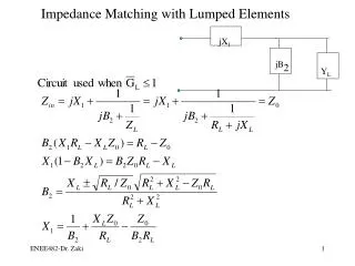
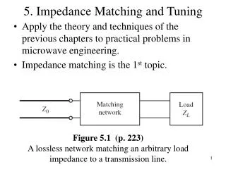
5. Impedance Matching and Tuning. Apply the theory and techniques of the previous chapters to practical problems in microwave engineering. Impedance matching is the 1 st topic. Figure 5.1 (p. 223) A lossless network matching an arbitrary load impedance to a transmission line.

E N D
5. Impedance Matching and Tuning • Apply the theory and techniques of the previous chapters to practical problems in microwave engineering. • Impedance matching is the 1st topic. Figure 5.1 (p. 223)A lossless network matching an arbitrary load impedance to a transmission line.
Impedance matching or tuning is important since • Maximum power is delivered when the load is matched to the line, and power loss in the feed line is minimized. • Impedance matching sensitive receiver components improves the signal-to-noise ratio of the system. • Impedance matching in a power distribution network will reduce the amplitude and phase errors.
Important factors in the selection of matching network. • Complexity • Bandwidth • Implementation • Ajdustability
5.1 Matching with Lumped Elements • L-section is the simplest type of matching network. • 2 possible configurations Figure 5.2 (p. 223)L-section matching networks. (a) Network for zL inside the 1 + jx circle. (b) Network for zL outside the 1 + jx circle.
Analytic Solution • For Fig. 5. 2a, let ZL=RL+jXL. For zL to be inside the 1+jx circle, RL>Z0. For a match, • Removing X
Smith Chart Solutions • Ex 5.1
Figure 5.3b (p. 227)(b) The two possible L-section matching circuits. (c) Reflection coefficient magnitudes versus frequency for the matching circuits of (b).
5.2 Single Stub Tuning Figure 5.4 (p. 229)Single-stub tuning circuits. (a) Shunt stub. (b) Series stub.
2 adjustable parameters • d: from the load to the stub position. • B or X provided by the shunt or series stub. • For the shunt-stub case, • Select d so that Y seen looking into the line at d from the load is Y0+jB • Then the stub susceptance is chosen as –jB. • For the series-stub case, • Select d so that Z seen looking into the line at d from the load is Z0+jX • Then the stub reactance is chosen as –jX.
Shunt Stubs • Ex 5.2 Single-Stub Shunt Tuning ZL=60-j80 Figure 5.5a (p. 230)Solution to Example 5.2. (a) Smith chart for the shunt-stub tuners.
Figure 5.5b (p. 231)(b) The two shunt-stub tuning solutions. (c) Reflection coefficient magnitudes versus frequency for the tuning circuits of (b).
To derive formulas for d and l, let ZL= 1/YL= RL+ jXL. • Now d is chosen so that G = Y0=1/Z0,
If RL = Z0, then tanβd = -XL/2Z0. 2 principal solutions are • To find the required stub length, BS = -B. for open stub for short stub
Series Stubs • Ex 5.3 Single Stub Series Tuning ZL = 100+j80 Figure 5.6a (p. 233)Solution to Example 5.3. (a) Smith chart for the series-stub tuners.
Figure 5.6b (p. 232)(b) The two series-stub tuning solutions. (c) Reflection coefficient magnitudes versus frequency for the tuning circuits of (b).
To derive formulas for d and l, let YL= 1/ZL= GL+ jBL. • Now d is chosen so that R = Z0=1/Y0,
If GL = Y0, then tanβd = -BL/2Y0. 2 principal solutions are • To find the required stub length, XS = -X. for short stub for open stub
5.3 Double-Stub Tuning • If an adjustable tuner was desired, single-tuner would probably pose some difficulty. Smith Chart Solution • yL add jb1 (on the rotated 1+jb circle) rotate by d thru SWR circle(WTG) y1 add jb2 Matched • Avoid the forbidden region.
Figure 5.7 (p. 236)Double-stub tuning. (a) Original circuit with the load an arbitrary distance from the first stub. (b) Equivalent-circuit with load at the first stub.
Figure 5.8 (p. 236)Smith chart diagram for the operation of a double-stub tuner.
Figure 5.9a (p. 238)Solution to Example 5.4. (a) Smith chart for the double-stub tuners. Ex. 5.4 ZL = 60-j80 Open stubs, d = λ/8
Figure 5.9b (p. 239)(b) The two double-stub tuning solutions. (c) Reflection coefficient magnitudes versus frequency for the tuning circuits of (b).
Analytic Solution • To the left of the first stub in Fig. 5.7b, Y1 = GL + j(BL+B1) where YL = GL + jBL • To the right of the 2nd stub, • At this point, Re{Y2} = Y0
Since GL is real, • After d has been fixed, the 1st stub susceptance can be determined as • The 2nd stub susceptance can be found from the negative of the imaginary part of (5.18)
B2 = • The open-circuited stub length is • The short-circuited stub length is
5.4 The Quarter-Wave Transformer • Single-section transformer for narrow band impedance match. • Multisection quarter-wave transformer designs for a desired frequency band. • One drawback is that this can only match a real load impedance. • For single-section,
Figure 5.10 (p. 241)A single-section quarter-wave matching transformer. at the design frequency f0.
The input impedance seen looking into the matching section is where t = tanβl = tanθ, θ = π/2 at f0. • The reflection coefficient • Since Z12 = Z0ZL,
Now assume f ≈ f0, then l ≈ λ0/4 and θ ≈ π/2. Then sec2 θ >> 1.
We can define the bandwidth of the matching transformer as • For TEM line, • At θ = θm,
The fractional bandwidth is • Ex. 5.5 Quarter-Wave Transformer Bandwidth ZL = 10, Z0 = 50, f0= 3 GHz, SWR ≤ 1.5
Figure 5.12 (p. 243)Reflection coefficient magnitude versus frequency for a single-section quarter-wave matching transformer with various load mismatches.
5.5 The Theory of Small Reflection Single-Section Transformer
Figure 5.13 (p. 244)Partial reflections and transmissions on a single-section matching transformer.
Multisection Transformer • Assume the transformer is symmetrical,
If N is odd, the last term is while N is even,
5.6 Binomial Multisection Matching Transformer • The response is as flat as possible near the design frequency. maximally flat • This type of response is designed, for an N-section transformer, by setting the first N-1 derivatives of |Γ(θ)| to 0 at f0. • Such a response can be obtained if we let
Note that |Γ(θ)| = 0 for θ=π/2, (dn |Γ(θ)|/dθn ) = 0 at θ=π/2 for n = 1, 2, …, N-1. • By letting f 0,
Γn must be chosen as • Since we assumed that Γn are small, ln x ≈ 2(x-1)/(x+1), • Numerically solve for the characteristic impedance Table 5.1
The bandwidth of the binomial transformer • Ex. 5.6 Binomial Transformer Design
Figure 5.15 (p. 250)Reflection coefficient magnitude versus frequency for multisection binomial matching transformers of Example 5.6 ZL = 50Ω and Z0 = 100Ω.
5.7 Chebyshev Multisection Matching Transformer Chebyshev Polynomial • The first 4 polynomials are • Higher-order polynomials can be found using
Figure 5.16 (p. 251)The first four Chebyshev polynomials Tn(x).
Properties • For -1≤x ≤1, |Tn(x)|≤1 Oscillate between ±1 Equal ripple property. • For |x| > 1, |Tn(x)|>1 Outside the passband • For |x| > 1, |Tn(x)| increases faster with x as n increases. • Now let x = cosθ for |x| < 1. The Chebyshev polynomials can be expressed as More generally,
We need to map θmto x=1 and π- θm to x = -1. For this, • Therefore,
Design of Chebyshev Transformers • Using (5.46) • Letting θ = 0,
If the maximum allowable reflection coefficient magnitude in the passband is Γm,