Download
1 / 31
340 likes | 517 Vues
Explore various types of cost estimation models such as Experiential, Static, and Dynamic, including techniques like Expert Guessing, Delphi Technique, and Wolverton Model in software cost estimation. Learn about the challenges of expert judgment, parameter estimation, function points, and static linear models. Discover the assumptions, equations, and models of Halstead’s Software Science, Watson and Felix, Bailey and Basili, and COCOMO. Dive into dynamic models like Putnam Model for accurate project effort estimation.

E N D
Cost Estimation CIS 375 Bruce R. Maxim UM-Dearborn
Types of Cost Models • Experiential • derived from past experience • Static • derived using “regression” techniques • doesn’t change with time • Dynamic • derived using “regression” techniques • often includes the effects of time
Expert Guessing A = The most pessimistic estimate. B = The most likely estimate. C = The most optimistic estimate. Ê = (A + 4B + C) 6 (Weighted average; where Ê = estimate).
Delphi Technique • Group of experts, make "secret" guesses. • "secret" guesses are used to compute group average. • Group average is presented to the group. • Group, once again makes "secret" guesses. • Individual guesses are again averaged. • If new average is different from previous, then goto (4). • Otherwise Ê = new average.
Wolverton Model - 1 Uses a software type matrix where the column headings come from the cross product {old, new} X {easy, moderate, hard} For example:
Wolverton Model -2 • Estimate models in terms of LOC: C(k) = Ss(k) * Ci,j(k) Cost of = Size matrix cost entry module k = of module k for modules like K System Cost = C(k) where k = 1 to n
Problems with Expert Judgement • It is subjective. (consensus is difficult to achieve) • Extrapolating from one project to another may be difficult. • Users and project managers tend not to estimate costs very well. • Cost matrices require periodic updates.
Parameter Simple + Average + Complex = Fi Distinct input items 3( ) + 4( ) + 6( ) = ? Output screens/reports 4( ) + 5( ) + 7( ) = ? Types of user queries 3( ) + 4( ) + 6( ) = ? Number of files 7( ) + 10( ) + 15( ) = ? External interface 5( ) + 7( ) + 10( ) = ? Total = ? Function Points
Function Point Equation F.P.’s = T * (0.65 + 0.01 * Q) T = unadjusted table total Q = score from questionnaire (14 items with values 0 to 5) • Cost of producing one function point? May be organization specific.
Backup. Data communication. Distributed processes. Optimal performance. Heavily used operating system. On-line data security. Multiple screens. On-line master file update. Complex inputs, queries, outputs. Complex internal processing. Reusable code. Conversion or installation. Multiple user sites. Ease of use. Function Point Questionnaire
Static Linear Models Often built using regression analysis Effort = c0 + ci * xi C = regression coefficient X = product or process attribute
Static Non-Linear Models Examples Effort = c0 + ci * xidi Cianddi are non-linear regression constants or Effort = (a + b S C) * m(X) where S is size in KLOC a, b, and c are regression constants
Halstead’s Software Science Assumptions • complete algorithm specification exists • programmer works alone • programmer knows what to do • Based on N = # of unique operators n = # of unique operands
Halstead Equations Effort E = N2 * log2 (n) / 4 To compute N N = k * Ss k = average # operators per LOC k is language specific To compute n N = n * log2 (n / 2)
Watson and Felix Model E = 5.25 * S 0.91 composite productivity factor p = wi * xi L = LOC per person-month = f(p) E = S / L
Bailey and Basili Model E` = 5.5 + 0.73 * S 1.6 R = E / E’ = actual effort/predicted effort Adjusted effort is ERadj = R – 1 if R >= 1 = 1 – 1/R if R < 1 Eadj = (1 + ERadj) * E if R >= 1 = E / (1 + ERadj) if R < 1
BASIC INTERMEDIATE MODE a b a b Organic 2.4 1.05 3.2 1.05 Semidetached 3.0 1.12 3.0 1.12 Embedded 3.6 1.20 2.8 1.20 COCOMO - I • Model E = a Sb * m(x)
Basic COCOMO • Computes software development effort (and cost) as a function of program size, expressed in estimated lines of code. • m(x) = 1
Intermediate COCOMO • Computes software development effort as a function of program size and a set of "cost drivers" that include subjective assessments of product, hardware, personnel, and project attributes. • m(x) = m(xi)
Detailed COCOMO • Includes all characteristics of the intermediate version with an assessment of the cost driver’s impact on each step (analysis, design, ect.) of the software engineering process • m(x) based on similar questionnaire
Static Model Problems • Existing models rely at least in part on expert judgment • Most static estimates require estimation of the product in lines of code (LOC) • Not clear which cost factors are significant in all development environments
Dynamic Models • It is helpful to know when effort will be required on a project as well as how much total effort is required • Most models are time or phase sensitive in their effort computations
Putnam Model Based on Rayliegh curve - > skewed, median & mean offset from one another
Putnam Model Details • Volume of work • Difficulty gradient for measuring complexity • Project technology factor measuring staff experience • Delivery time constraints • Staffing model based on • Total cumulative staff • How quickly new staff can be absorbed • # days in project month
Putnam Equations E = y(T) = 0.3945 * K K = area under curve [0 , 1) measured in programmer year T = optimal development time in years D = K / T2 difficulty P = ci * D –2/3productivity S = c * K –1/3 * T 4/3 lines of code
Parr Equation • Putnam variation • Staff may already be familiar with project tools, methods, and requirements Staff(t) = (sech2 (a*t + c) / 2) / 4
Jensen Model • Putnam variation • Less sensitive to schedule compression than Putnam S = Cte * T * K1/2
Cooperative Programming Model • Includes size of project team in estimate as well as code size E = E1(S) + E2(M) S = code size M = average # team members E1(S) = a + b * S effort of single team member E2(M) = c * Md effort required for coordination with other members
Dynamic Model Problems • Still rely on expert judgment • Not clear that all project costs have been accommodated here either