Atomic Structure and Atomic Spectra (CH 13)

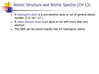
1. Atomic Structure and Atomic Spectra (CH 13) • A hydrogenic atom is a one-electron atom or ion of general atomic number Z; H, He+, Li2+,… • A many-electron atom is an atom or ion with more than one electron. • The SWE can be solved exactly only for hydrogenic atoms.

2. Atomic Spectra of H atoms • The atomic emission of excited H atoms gives a line spectra. • Johann Balmer noted that the wavenumbers of the these lines fit the expression: • These emissions are now called the Balmer series.

3. Atomic Spectra of H atoms • The atomic emission of excited H atoms gives a line spectra. • Additional lines were discovered in the UV and the infrared and Rydberg noted that the lines fit the general expression. • Different values of n1 give a series of lines: • n1=1 (Lyman series) n2=2,3,4,… • n1=2 (Ballmar series) n2=3,4,5,… • n1=3 (Paschen series) n2=4,5,6,…

4. Atomic Spectra of H atoms • Energy is conserved when a photon is emitted, so the difference in energy of the atom before and after the emission event must be equal to the energy of the photon emitted. • Therefore, the n1 & n2 integers in the Rydberg equation must correspond to quantum numbers for the hydrogen atom.

5. Atomic Spectra of H atoms Visible Emissions Infrared emissions UV emissions

6. Atomic # Elementary charge Distance from the nucleus Vacuum permittivity The SWE for Hydrogenic Atoms • The potential energy for an electron in a hydrogenic atom is due to coulombic attraction between the electron and the nucleus.

7. The SWE for Hydrogenic Atoms • The Hamiltonian must have terms for the KE of the nucleus, KE of electron, and any potential energy. • We can separate the relative motion of the electron and the nucleus from the motion of the atom as a whole giving two equations: • One describing the free translational motion of a particle of mass m=me+mN. We’ve already solved this problem in CH 11. • One describing the internal motion of the electron relative to the nucleus. • From now on, we’ll speak only in terms of the internal, relative coordinates.

8. The SWE for Hydrogenic Atoms • The potential energy is independent of angle allowing the wave function to be seperable into radial and angular components. Y(r,q,f)=R(r)Y(q,f) • Results in two separate diff equations to solve: • The particle on a sphere is the solution to the angular part. • Now we just need the solution to the radial part.

9. The Radial Part of the SWE • Write the Hamiltonian. • Define Veff. • For zero orbital angular momentum, Veff = Coulombic potential energy. • For nonzero orbital angular momentum, the centrifugal effect gives rise to a positive contribution which is very large near the nucleus.

10. The Radial Solution • Solving the radial equation gives energies: • The wavefunctions are shown in table 13.1, p. 349.

11. The Radial Wavefunctions

12. Atomic Orbitals • An atomic orbital is a one-electron wavefunction for an electron in an atom. • Each AO is defined by three quantum numbers: n, l, ml Principal quantum number: n = 1,2,3,… {Determines the energy} Angular momentum quantum number: l=0,1,2,…,n-1 Magnetic quantum number: ml=l,l-1,l-2,…,-l

13. Atomic Energy Levels • The energy levels are determined by the principal quantum number: • Gives almost exact agreement with experimental values. Disagreement arises from relativistic effects, which are not treated by the non-relativistic SWE. • Each energy level is n2-fold degenerate due to the different possible values for l and ml. • Selection rules only allow certain transitions to occur:

14. Atomic Energy Levels • We arbitrarily define an infinitely separated atom and electron to have zero energy. • Negative energy implies a bound state. • The energy of the atom is lower than that of an infinitely separated stationary electron and nucleus. • Positive energy corresponds to an unbound state. • The energies of an unbound electron are not quantized and therefore form a continuum of states. • The ionization energy is the minimum amount of energy required to remove an electron from the ground state to the continuum.

15. Shells and Subshells • An orbital with a given value of n forms a single shell of the atom. • Shells are referred to by letters: n = 1 2 3 4 K L M N Orbitals with the same n, but different values of l form subshells. l = 0 1 2 3 4 5 6 s p d f g h i

16. Shells and Subshells

17. s orbitals • All s orbitals are spherically symmetric becauses there’s no angular dependence in Y0,0(q,f). (See table 12.3 p. 334) • There are radial nodes where the polynomial factor (see table 13.1 p. 349) is equal to zero. • Demonstrate for 2s orbital:

18. Electron probability density • It is common to depict the probability density of the electron |Y|2 by the density of shading. • On the left, we have the probability density of a 1s and 2s orbital. Note the node in the 2s orbital.

19. Boundary Surface (Size of an orbital) • Sometimes the size of an orbital is represented as a boundary surface, the surface that captures about 90% of the the electron probability.

20. Orbital Size • What is the mean radius of a 1s orbital? • In general: • Average radius increases as n increases. • For a given value of n, the mean radius lies in the order d < p < s.

21. Radial Distribution Functions • The probability of finding an electron in any region is given through |Y|2. • But consider the probability of finding the electron anywhere on a spherical shell of thickness dr at a radius r. • P(r)dr gives the probability of finding the electron anywhere in this shell and is termed the radial distribution function.

22. Radial Distribution Functions for 1s orbital • Define P(r) for a 1s orbital. • P(0)=0; P(r)0 as rinfinity • Find the most probable radius for a 1s electron.

23. p orbitals • For nonzero l, the centrifugal effect goes to infinity as r goes to zero. • This causes the potential energy to go to infinity at r=0. • There’s therefore no probability of the electron being at the nucleus. • Show the three p orbitals, which are distinguised by three different values for ml.

24. z pz orbital • The xy-plane is the nodal plane, hence the origin of the “pz-orbital”. • Although the density is positive everywhere, different shading indicates the phase of Y.

25. px and Py orbitals • These are obtained by taking linear combination of the P+1 and P-1. • The result gives real functions which are still valid solutions to the SWE. Show.

26. d orbitals • d orbitals are formed the same way, by taking linear combinations of the oribitals with opposite values of ml.

27. Selection Rules • Photons are bosons and have s=1. • This angular momentum must be conserved when a photon is produced (emitted) or destroyed (absorbed). • For this conservation to occur Dl=±1. • An electron in a d orbital (l=2) cannot make a transition into an s orbital (l=0) because the photon cannot carry away enough angular momentum. • An s electron cannot make a transition to another s orbital because the no angular momentum is produced for the photon. • n is unrestricted because it doesn’t relate to angular momentum.

28. Transition Dipole Moment • The rate of transition is equivalent to either: • The intensity of absorption of light OR • The intensity of emission of light • The rate is proportional to the square of the transition dipole moment. • Physically, the transition dipole moment is a measure of the ‘kick’ the electron gives to or receives from the electromagnetic field. • The derivation of the transition dipole moment comes from time dependent perturbation theory. • Define time dependent SWE. • Deine the perturbation.

29. Grotrian Diagrams • A Grotrian diagram summarizes the energies of the states and the transitions between them. • This the Grotrian diagram for hydrogen.

30. The structure of many-electron atoms • The wavefunction of a many-electron atom is a very complicated function of the coordinates of all the electrons. • Y(r1,r2,…ri) where riis the vector from the nucleus to electron i. • In the orbital approximation we assume that the electrons don’t interact, then the wavefunction can be written as a product of orbitals for each electron.

31. Pauli Principle • The Pauli exclusion principle says that no more than two electrons may occupy a given orbital, and if two do occupy one orbital, then their spins must be paired. • So for Li (Z=3) the first two electrons fill the 1s orbital and the third will go elsewhere. • Comes from the more general Pauli Principle. • The Pauli Principle states says that when two labels of any two fermions are exchanged, the total wavefunction must change sign and when two labels of any two bosons are exchanged the total wavefunction must NOT change signs.

32. Many-electron atoms subshell energies • In many electron atoms, the 2s and 2p orbitals are generally not degenerate. WHY? • The 1s electrons repel the n=2 electrons. • The nuclear charge is shielded by the 1s electrons giving rise to an effective nuclear charge: zeff = z – s • The shielding constant s is different for 2s and 2p orbitals because they have different radial distribution functions. • An s electron has greater penetration through the inner shells so is shielded less. • As a consequence of nuclear shielding, the subshell energies lie: s<p<d<f.

33. Aufbau “building up” principle • The Aufbau principle says that electrons will fill the lowest energy orbitals first (each holding two electrons). 1s 2s 2p 3s 3p 4s 3d 4p 5s • The complicated order comes from the electron-electron repulsion which is important when orbitals have almost the same energy (4s & 3d). • Example: Using the orbital approximation, give the wavefunction for a carbon atom (Z=6).

34. Hund’s rule • An atom in its ground state adopts a configuration with the greatest number of unpaired electrons. • Hund’s rule comes from spin correlation which keeps parallel spinning electrons apart causing them to repel less. • Proof: Consider a two electron system w/ each electron in a two different degenerate orbitals. • The antisymmetric wavefunction vanishes if r1=r2. • The symmetric wavefunctions do not vanish. • Consequently, two electrons have different relative spatial distributions depending on whether their spins are parallel or not. • Different spatial distributions means different Coulombic interactions and states with different energies. • States with electrons having parallel spin will be lower in energy and will fill first.

35. Quantum Defects and Rydberg States • The energy of many electron atoms does not generally vary as 1/n2, but the energies of outermost electrons do if we account for shielding by the other Z-1 electrons. • The binding energies of these electrons will be of the form ? (Recall Rydberg), but will be slightly lower in energy due to the Zeff being slightly larger than 1. • Introduce quantum defectd as a fudge factor. • For very diffuse states, 1/n2 variation is valid. These states are called Rydberg states.

36. Spin Orbit Coupling • Spin-orbit coupling is best explained in terms of total angular momentum—a vector sum of orbital and spin angular momentum. j=l+1/2 {same direction} j=l-1/2 {opposite direction}

37. Spin-orbit coupling constant Spin Orbit Coupling • The magnetic field generated by a spinning electron interacts with the magnetic field generated by the orbiting electron. • This causes a further splitting of the energy levels.

38. Strength of Spin-Orbit Coupling • The strength of Spin-Orbit Coupling depends on the nuclear charge. • Imagine riding on an electron and seeing the nucleus orbit around you (much like the sun rising and setting). • Since the ‘sun’ is charged, you would be at the center of a ring of current. • The higher the charge, the greater the current, and therefore the stronger the magnetic field induced by the current on you. • The magnetic field from this orbital motion interacts with the magnetic moment on the electron. • As Z increases, the spin-orbit coupling increases.

39. Spin-Orbit coupling and Fine Structure • Two spectral lines are observed when the p electron of an electronically excited alkali metal atom undergoes a transition and falls into a lower s orbital. • One line is due to a transtion from a j=3/2 level. • One line is due to a transition from a j=1/2 level. • The two observed lines are called fine structure and are due to spin-orbit coupling. The Na D lines

40. Term Symbols • A term symbol conveys all the information the angular momentum quantum numbers of an atom (or molecule). • Lower case letters are used to label orbitals, upper case letters are used to label overall states. • We now of three quantum numbers associated with angular momentum: • Spin angular momentum • Orbital angular momentum • A closed shell has zero orbital angular momentum because all the individual orbital angular momenta sum to zero. • Total angular momentum • Example: Write the possible terms arising from 1s22s12p1 configuration.

41. Russel-Saunders coupling vs. jj-coupling • Russell –Saunders Coupling • Assumes no coupling between individual electron’s angular and spin momenta. • J is from sum of all L and S. • Work’s for light atoms. • jj – coupling • Spin and orbital momentum of each electron is coupled strongly. • Must treat electron as particle with angular momentum j. • S and L are not ‘true’ quantum numbers, only J. • Selection rules for DS can be broken in heavy atoms because only DJ selection rule is valid.

42. Summary of all the energy level splitting.

43. The Zeeman Effect • Further splitting can be caused if an atom is placed in a strong magnetic field. • States with different mlvalues will interact differently with the magnetic field, lifting their degeneracies. • Additional splitting can occur due to the magnetic moment of the spinning electrons.

44. Variational Method • The orbital approximation is crude and gives energies that are much too low since electron repulsion is neglected. • We can use the variational method to obtain a better wavefunction. • If Y is a well-behaved function of the coordinates then • If Y is the true ground state energy wavefunction, then the equality applies. • Otherwise we use an approximate wavefunction (having correct boundary conditions), known as a trial wavefunction. The variational energy will always be higher than the true ground state energy.

45. Calculation of the Variational Energy • A trial wavefunction that satisfies the boundary conditions for a particle in a box is Y=x(L-x). Calculate the variational energy for this function and show that it’s greater then Eg.s.

46. Variational Method • We can add adjustable parameters to our trial wavefunction. • The parameters are adjusted such to minimize our energy giving a result that is closer to the true ground state energy. • For the helium atom, a good trial function would be Y=1s(1)1s(2)=? • We could replace Z with Zeff = z – s to account for electron shielding and calculate the variational energy (which will be function of s). • Solving for s that minimizes the variational energy will be an upper bound to the ground state energy. • Eg.s. (experimental) = -79.0 eV • This method = -77.5 eV • Not bad considering we’ve only adjusted one parameter. • We can use more parameters or change the form of the the trial function to get an energy that is even closer to the “true” value.

47. Variational Method Limitations • This method becomes impractical as the number of electrons increases because of the complicated electron-electron repulsion term that must be integrated.