Disjoint Sets

1. Disjoint Sets Andreas Klappenecker [Based on slides by Prof. Welch]

2. Dynamic Sets In mathematics, a set is understood as a collection of clearly distinguishable entities (called elements). Once defined, the set does not change. In computer science, a dynamic set is understood to be a set that can change over time by adding or removing elements.

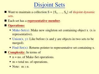
3. Abstract Data Type: Disjoint Sets • State: collection of disjoint dynamic sets • The number of sets and their composition can change, but they must always be disjoint. • Each set has a representative element that serves as the name of the set. • For example, S={a,b,c} can be represented by a. • Operations: • Make-Set(x): creates singleton set {x} and adds it the to collection of sets. • Union(x,y): replaces x's set Sx and y's set Sy with Sx U Sy • Find-Set(x): returns (a pointer to) the representative of the set containing x

4. Disjoint Sets Example • Make-Set(a) • Make-Set(b) • Make-Set(c ) • Make-Set(d) • Union(a,b) • Union(c,d) • Find-Set(b) • Find-Set(d) • Union(b,d) b a c d returns a returns c

5. Example The Disjoint Sets data structure can be used in Kruskal’s MST algorithm to test whether adding an edge to a set of edges would cause a cycle. Recall that in Kruskal’s algorithm the edges chosen so far form a forest. The basic idea is to represent each connected component of this forest by its set of vertices. In other words, each dynamic set represents a tree.

6. Example (continued) Initially, form the singleton sets {v1}, …, {vn}. • For all vertices v in V do Make-Set(v). od. Add an edge unless this would form a cycle: • For all edges e=(u,v) taken in increasing weight do Union(u,v) unless Find-Set(u)=Find-Set(v). od.

7. Disjoint Sets in Linked List Representation

8. Dynamic Sets in Linked List Representation Idea: Store the set elements in a linked list. Each list node has a pointer to the next list node The first list node is the set representative rep. Each list node also has a pointer to the set representative rep. Keep external pointers to first list node (rep) and last list node (tail)

9. e d a f b c rep tail rep tail rep tail Linked List Representation

10. Linked List Representation • Make-Set(x): make a new linked list containing just a node for x • O(1) time • Find-Set(x): given (pointer to) linked list node containing x, follow rep pointer to head of list • O(1) time • Union(x,y): append list containing x to end of list containing y and update all rep pointers in the old list of x to point to the rep of y. • O(size of x's old list) time

11. Time Analysis • What is worst-case time for any sequence of Disjoint Set operations, using the linked list representation? • Let m be number of operations in the sequence • Let n be number of Make-Set operations (i.e., number of elements)

12. Expensive Case Consider the sequence of operations: • Make-Set(x1), Make-Set(x2), …, Make-Set(xn), Union(x1,x2), Union(x2,x3), …, Union(xn-1,xn) This sequences contains m=2n-1 operations. The total time these m operations is O(n2), since unions update 1,2,…,n-1 elements. We have O(n2)=O(m2) since m = 2n – 1. Thus, the amortized time per operation is O(m2)/m = O(m).

13. Partial Remedy: Linked List with Weighted Union • Always append smaller list to larger list • Need to keep count of number of elements in list (weight) in rep node We will now calculate the worst-case time for a sequence of m operations. Clearly, the Make-Set and Find-Set operations contribute O(m) total. The Union operations are more critical.

14. Analyzing Time for All Unions How many times must the rep pointer for an arbitrary node x be updated? • The first time the rep pointer of x is updated, the new set has at least 2 elements. • The second time rep pointer of x is updated, the new set has at least 4 elements. [Indeed, the set containing x has at least 2 elements and the other set is at least as large as the set containing x.]

15. Analyzing Time for All Unions • The maximum size of a set is n (the number of Make-Set ops in the sequence) • So the rep pointer of x may be updated at most log n times. • Thus total time for all unions is O(n log n). • Note the style of counting - focus on one element and how it fares over all the Unions

16. Amortized Time • Grand total for sequence is O(m+n log n) • Amortized cost per Make-Set and Find-Set is O(1) • Amortized cost per Union is O(log n) since there can be at most n - 1 Union ops.

17. Disjoint Sets in Tree Representation

18. Tree Representation • Can we improve on the linked list with weighted union representation? • Use a collection of trees, one per set • The rep is the root • Each node has a pointer to its parent in the tree

19. a d e b f c Tree Representation

20. Analysis of Tree Implementation • Make-Set: make a tree with one node • O(1) time • Find-Set: follow parent pointers to root • O(h) time where h is height of tree • Union(x,y): make the root of x's tree a child of the root of y's tree • O(1) time • So far, no better than original linked list implementation

21. Improved Tree Implementation • Use a weighted union, so that smaller tree becomes child of larger tree • prevents long chains from developing • can show this gives O(m log n) time for a sequence of m ops with n Make-Sets • Also do path compression during Find-Set • flattens out trees even more • can show this gives O(m log*n) time!

22. Interlude: What is log*n ? • The number of times you can successively take the log, starting with n, before reaching a number that is at most 1 • More formally: • log*n = min{i ≥ 0 : log(i)n ≤ 1} • where log(i)n = n, if i = 0, and otherwise log(i)n = log(log(i-1)n)

23. Examples of log*n

24. log*n Grows Slowly • For all practical values of n, log*n is never more than 5.

25. Make-Set • Make-Set(x): • parent(x) := x • rank(x) := 0 // used for weighted union

26. Union • Union(x,y): • r := Find-Set(x); s := Find-Set(y) • if rank(r) > rank(s) then parent(s) := r • else parent(r) := s • if rank(r ) = rank(s) then rank(s)++

27. Rank • gives upper bound on height of tree • is approximately the log of the number of nodes in the tree • Example: • MS(a), MS(b), MS(c), MS(d), MS(e), MS(f), • U(a,b), U(c,d), U(e,f), U(a,c), U(a,e)

28. d c b a f e End Result of Rank Example 2 1 0 1 0 0

29. Find-Set • Find-Set(x): • if x  parent(x) then • parent(x) := Find-Set(parent(x)) • return parent(x) • Unroll recursion: • first, follow parent pointers up the tree • then go back down the path, making every node on the path a child of the root

30. a b c d e e d c b a Find-Set(a)

31. Amortized Analysis • Show any sequence of m Disjoint Set operations, n of which are Make-Sets, takes O(m log*n) time with the improved tree implementation. • Use aggregate method. • Assume Union always operates on roots • otherwise analysis is only affected by a factor of 3

32. Charging Scheme • Charge 1 unit for each Make-Set • Charge 1 unit for each Union • Set 1 unit of charge to be large enough to cover the actual cost of these constant-time operations

33. Charging Scheme • Actual cost of Find-Set(x) is proportional to number of nodes on path from x to its root. • Assess 1 unit of charge for each node in the path (make unit size big enough). • Partition charges into 2 different piles: • block charges and • path charges

34. Overview of Analysis • For each Find-Set, partition charges into block charges and path charges • To calculate all the block charges, bound the number of block charges incurred by each Find-Set • To calculate all the path charges, bound the number of path charges incurred by each node (over all the Find-Sets that it participates in)

35. ranks: 0 1 2 3 4 5 … 16 17 … 65536 65537 … blocks: 0 1 2 3 4 5 Blocks • Consider all possible ranks of nodes and group ranks into blocks • Put rank r into block log*r

36. Charging Rule for Find-Set • Fact: ranks of nodes along path from x to root are strictly increasing. • Fact: block values along the path are non-decreasing • Rule: • root, child of root, and any node whose rank is in a different block than the rank of its parent is assessed a block charge • each remaining node is assessed a path charge

37. Find-Set Charging Rule Figure 1 block charge (root) block b'' > b' 1 block charge 1 path charge … 1 path charge block b' > b … 1 block charge 1 path charge block b 1 block charge … 1 path charge

38. Total Block Charges • Consider any Find-Set(x). • Worst case is when every node on the path from x to the root is in a different block. • Fact: There are at most log*n different blocks. • So total cost per Find-Set is O(log*n) • Total cost for all Find-Sets is O(m log*n)

39. Total Path Charges • Consider a node x that is assessed a path charge during a Find-Set. • Just before the Find-Set executes: • x is not a root • x is not a child of a root • x is in same block as its parent • As a result of the Find-Set executing: • x gets a new parent due to the path compression

40. Total Path Charges • x could be assessed another path charge in a subsequent Find-Set execution. • However, x is only assessed a path charge if it's in same block as its parent • Fact: A node's rank only increases while it is a root. Once it stops being a root, its rank, and thus its block, stay the same. • Fact: Every time a node gets a new parent (because of path compression), new parent's rank is larger than old parent's rank

41. Total Path Charges • So x will contribute path charges in multiple Find-Sets as long as it can be moved to a new parent in the same block • Worst case is when x has lowest rank in its block and is successively moved to a parent with every higher rank in the block • Thus x contributes at most M(b) path charges, where b is x's block and M(b) is the maximum rank in block b

42. Total Path Charges • Fact: There are at most n/M(b) nodes in block b. • Thus total path charges contributed by all nodes in block b is M(b)*n/M(b) = n. • Since there are log*n different blocks, total path charges is O(n log*n), which is O(m log*n).

43. Even Better Bound • By working even harder, and using a potential function analysis, can show that the worst-case time is O(m(n)), where  is a function that grows even more slowly than log*n: • for all practical values of n, (n) is never more than 4.

44. Effect on Running Time of Kruskal's Algorithm • |V| Make-Sets, one per node • 2|E| Find-Sets, two per edge • |V| - 1 Unions, since spanning tree has |V| - 1 edges in it • So sequence of O(E) operations, |V| of which are Make-Sets • Time for Disjoint Sets ops is O(E log*V) • Dominated by time to sort the edges, which is O(E log E) = O(E log V).