
SlideServe
Menu
Préférences
© SlideServe · v2026

6.6

parry avatar
12 diapositives · 300 Views · Sep 08, 2014

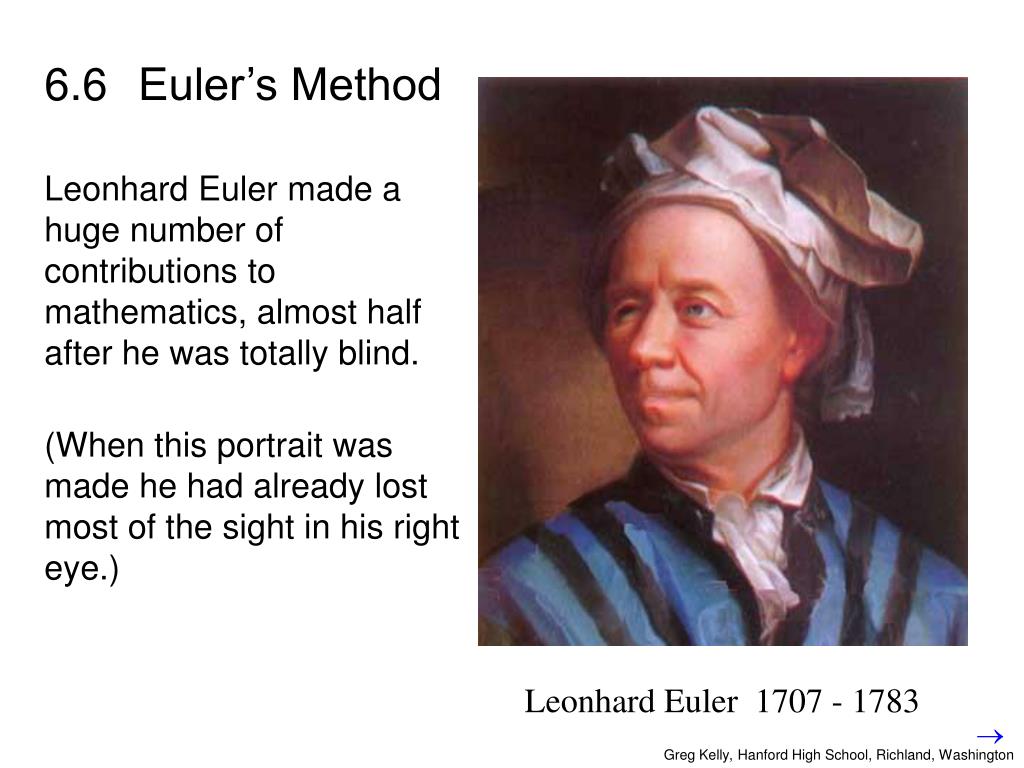
6.6. Euler’s Method. Leonhard Euler made a huge number of contributions to mathematics, almost half after he was totally blind. (When this portrait was made he had already lost most of the sight in his right eye.). Leonhard Euler 1707 - 1783.
6.6 - slide 1
01 / 126.6
1 / 17

Télécharger la présentation

6.6
Une image / un lien ci-dessous est fourni (tel quel) pour télécharger la présentation

Politique de téléchargement : le contenu du site vous est fourni TEL QUEL pour votre information et votre usage personnel ; il ne peut être vendu, concédé sous licence ni partagé sur d’autres sites sans l’accord de son auteur.Le contenu vous est fourni TEL QUEL, pour votre information et votre usage personnel uniquement. Téléchargez la présentation en cliquant sur ce lien. Lors du téléchargement, si vous ne parvenez pas à télécharger une présentation, l’éditeur a peut-être supprimé le fichier de son serveur.Pendant le téléchargement, si vous ne parvenez pas à obtenir une présentation, le fichier a peut-être été supprimé par l’éditeur.

F I N

Plus de contenu associé

Transcription de la présentation
  1. 6.6 Euler’s Method Leonhard Euler made a huge number of contributions to mathematics, almost half after he was totally blind. (When this portrait was made he had already lost most of the sight in his right eye.) Leonhard Euler 1707 - 1783 Greg Kelly, Hanford High School, Richland, Washington

  2. (function notation) (base of natural log) (pi) (summation) (finite change) It was Euler who originated the following notations: Leonhard Euler 1707 - 1783

  3. We will practice with an easy one that can be solved. There are many differential equations that can not be solved. We can still find an approximate solution. Initial Value: (0, 1) But first… Suppose we couldn’t solve this conventionally…

  4. Remember how it all started? Suppose we took the limit out. How would that change this? for very small dx values. Now let’s do a little algebra Which brings us to…

  5. Euler’s Method of Approximations So if we know , we have a value for and we have an initial value Then by Euler’s Method: BUT WHAT DOES IT ALL MEAN!?

  6. We will practice with an easy one that can be solved. There are many differential equations that can not be solved. We can still find an approximate solution. Initial Value: (0, 1) But first… Suppose we couldn’t solve this conventionally…

  7. So we have an approximate coordinate(0.5, 1) How could we use this to approximate

  8. So how would this compare to the real solution? How could we make the approximation better? Answer: A smaller dx value Try that in the Euler program on your calculator.

  9. Again, the real use of Euler’s Method is for differential equations that we can’t immediately solve. 1 3 2 Like, say, this one: 1.2 2.6 3.8 1.4 4.76 3.36 1.6 5.91 4.312 1.8 7.29 5.494 2 8.95 6.953 Approximate y(2) Remember:

  10. The actual solution to this is: Don’t worry about how? 1 3 2 Like, say, this one: 1.2 2.6 3.8 1.4 4.76 3.36 1.6 5.91 4.312 1.8 7.29 5.494 2 8.95 6.953 Approximate y(2) Use this solution to test your approximation on your calculator Remember:

  11. The calculator also contains a similar but more complicated (and more accurate) formula called the Runge-Kutta method. You don’t need to know anything about it other than the fact that it is used more often in real life. This is the RK solution method on your calculator. The book refers to an “Improved Euler’s Method”. We will not be using it, and you do not need to know it. p