Prof. Nicholas Zabaras
660 likes | 856 Vues
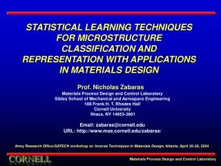
STATISTICAL LEARNING TECHNIQUES FOR MICROSTRUCTURE CLASSIFICATION AND REPRESENTATION WITH APPLICATIONS IN MATERIALS DESIGN. Prof. Nicholas Zabaras. Materials Process Design and Control Laboratory Sibley School of Mechanical and Aerospace Engineering 188 Frank H. T. Rhodes Hall

Prof. Nicholas Zabaras
E N D
Presentation Transcript
STATISTICAL LEARNING TECHNIQUES FOR MICROSTRUCTURE CLASSIFICATION AND REPRESENTATION WITH APPLICATIONS IN MATERIALS DESIGN Prof.Nicholas Zabaras Materials Process Design and Control Laboratory Sibley School of Mechanical and Aerospace Engineering188 Frank H. T. Rhodes Hall Cornell University Ithaca, NY 14853-3801 Email: zabaras@cornell.edu URL: http://www.mae.cornell.edu/zabaras/ Army Research Office/GATECH workshop on Inverse Techniques in Materials Design, Atlanta, April 26-28, 2004
Design LIGHT armor for SUPERIOR PERFORMANCE STATISTICAL LEARNING TOOLBOX PROGNOSIS - Life & response prediction REAL TIME CONTROL – Real time property analysis and control (during processing) SIMULATION MATCHING DESIGN – Predictive modeling of processes (AIM) Aircraft engines Understanding and blocking fracture by MSD MOTIVATION FOR MICROSTRUCTURE-SENSITIVE DESIGN • Critical hardware components in the aerospace, naval & automotive industry, armor/projectile design, require improved material response, performance robustness, increased utility & lifing, etc. • Introduce complex materials and process design solutions using physically-based mathematical and statistical techniques • Microstructure-sensitive design of: • fracture toughness, corrosion, elastic, creep, fatigue & other properties
PROCESS DESIGN ALGORITHMS • 1. Exact methods • (Sensitvities) • Heuristic methods STATISTICAL LEARNING TOOLBOX Training samples NUMERICAL SIMULATION OF MATERIAL RESPONSE Update data In the library • Multi-length • scale analysis • Polycrystalline • plasticity STATISTICAL LEARNING TOOLBOX Image • Functions: • Classification methods • Identify new classes ODF Associate data with a class; update classes Process controller Pole figures
DEFORMATION PROCESS DESIGN SIMULATOR Research Objectives: To develop a mathematically and computationally rigorous gradient-based optimization methodology for virtual materials process design that is based on quantified product quality and accounts for process targets and constraints. • Current capabilities: • Development of a general purpose continuum sensitivity method for the design of multi-stage industrial deformation processes • Deformation process design for porous materials • Design of 3D realistic preforms and dies • Extension to polycrystal plasticity based constitutive models with evolution of crystallographic • texture Initial guess Optimal preform
Material Process Design Simulator Preforming Stage Finishing Stage Objective Iteration number Preforming Stage Finishing Stage Unfilled cavity Fully filled cavity 8 S h e a r m o d u l u s ( M P a ) 3 8 2 . 5 8 E + 0 4 3 7 2 . 5 5 E + 0 4 7 6 2 . 5 1 E + 0 4 8 5 2 . 4 8 E + 0 4 4 2 . 4 5 E + 0 4 4 3 2 . 4 2 E + 0 4 6 3 7 2 2 . 3 8 E + 0 4 Nondimensionalized Objective function (x1e-03) 1 2 . 3 5 E + 0 4 5 8.0 6.0 S h e a r m o d u l u s ( M P a ) 4 8 2 . 5 9 E + 0 4 2 4 4.0 7 2 . 5 5 E + 0 4 6 6 2 . 5 2 E + 0 4 5 5 2 . 4 9 E + 0 4 2.0 3 0 2 4 6 8 1 0 1 2 4 2 . 4 5 E + 0 4 Iteration index 3 2 . 4 2 E + 0 4 7 0.0 2 2 . 3 9 E + 0 4 0 1 2 3 4 5 6 3 1 2 . 3 6 E + 0 4 PROCESS DESIGN CAPABILITIES DESIGN OBJECTIVE DESIGN OBJECTIVE Design the preforming die for a fixed volume of the workpiece (1100-Al) such that the variation in state in the product is a minimum Design the extrusion die for a fixed reduction such that the variation in state in the product at the exit is a minimum Initial die Optimal die 0 . 9 4 0 . 9 3 0 . 9 2 Objective 0 . 9 1 0 . 9 0 . 8 9 0 . 8 8 0 1 2 3 4 5 6 7 8 9 Iteration index DESIGN OBJECTIVE Evaluate preform of a porous material (2024- T351Al) for a given die shape such that the die cavity is completely filled DESIGN OBJECTIVE Design the preforming die for a fixed volume of the workpiece (1100-Al) such that the finishing die is completely filled Objective function (x1.0E-05) Iteration number
F B F F F F F F B B B o o e p * p (1) Single crystal plasticity (1) Continuum framework (2) State evolves for each crystal (2) State variable evolution laws The effectiveness of design for desired product properties is limited by the ability of phenomenological state-variables to capture the dynamics of the underlying microstructural mechanisms (3) Desired effectiveness in terms of state variables (3) Ability to tune microstructure for desired properties Polycrystal plasticity provides us with the ability to capture material properties in terms of the crystal properties. This approach is essential for realistic design leading to desired microstructure-sensitive properties MULTI-LENGTH SCALE DESIGN APPROACH Phenomenology Polycrystal plasticity Initial configuration Deformed configuration Initial configuration Deformed configuration s0 s n n0 s0 n0 Intermediate thermal configuration Stress free (relaxed) configuration Stress free (relaxed) configuration Need for polycrystalline analysis Multi length scale design approach The inverse problem “of tuning the microstructure for desired material response” is difficult due to the large number of microstructural degrees of freedom Solution: Microstructure model reduction
Real time microstructure analysis – metrology tools • Averaging principles • Reduced models • Digital library SYNERGY BETWEEN MICROSTRUCTURES & PROCESSING Materials design – optimization in reduced microstructural space Reduced order models for efficient microstructure representation Process design simulator Processing governs microstructure – impossible to verify exact microstructural features Real time control of processes through reduced order models & simulation matching design Sensing across length-scales and quantification of uncertainty Materials testing driven by design robustness limits
Fn+1 x = x(X, t; β) B0 X ~ Ω =Ω (r, t; L) POLYCRYSTAL PLASTICITY BASED APPROACH Micro problem driven by the velocity gradient L Macro problem driven by the macro-design variable β Bn+1 L = L (X, t; β) Polycrystal plasticity L = velocity gradient • Design variables (β) are macro • design variables • Die shapes • Preform shapes • Processing conditions • Etc. Design objectives are micro-scale averaged material/process properties
MICROSTRUCTURE REDUCED MODEL REPRESENTATION Method of snapshots Suppose we had a collection of data (from experiments or simulations) for the ODF: Solve the optimization problem Is it possible to identify a basis where such that it is optimal for the data represented as Eigenvalue problem where POD technique – Proper Orthogonal Decomposition
DECOMPOSITION OF THE VELOCITY GRADIENT Plane strain compression Uniaxial tension Shear Design vectorα = {α1, α2, α3, α4, α5} Design problem: Determine α so as to obtain desired properties in the final product.
Full model VALIDATION OF REDUCED-ORDER REPRESENTATION Uniaxial tension test α = {1,0,0,0,0} t = 0.1 s Reduced model (Basis II) Reduced model (Basis I) • Basis – I 3 POD modes from a uniaxial tension test with strain rate of 1s-1 for t=0.2 s • Basis – II 9 POD modes from five tests (αi= 1s-1 for the ith test, αj= 0, i ≠ j ) for t = 0.2 s
Bn+1 Sensitivity kinematic sub-problem Fn+1 Sensitivity thermal sub-problem L = L (X, t; β) B0 L = velocity gradient I + (Ls)n+1 x = x(X, t; β) Ls = design velocity gradient Sensitivity constitutive sub-problem Bn+1 ~ Ω =Ω (r, t; L) Sensitivity contact & friction sub-problem o x + x = x(X, t; β+Δ β) ~ 0 Ω + Ω = Ω (r, t; L+ΔL) r – orientation parameter o L + L = L (X, t; β+Δ β) o Fn+1 + Fn+1 MULTI-LENGTH SCALE SENSITIVITY ANALYSIS A micro-field – depends on a macro design parameter (and) the velocity gradient as The velocity gradient – depends on a macro design parameter Sensitivity of the velocity gradient – driven by perturbation to the macro design parameter Sensitivity of this micro-field driven by the velocity gradient
Current capabilities: • Multi-length scale analysis of material behavior • Development of a general purpose multi-length scale continuum sensitivity method for the design of microstructures • Polycrystal plasticity based constitutive models with evolution of crystallographic • texture • Reduced-order representation of microstructures • Classification of microstructures for better process and property selection Research Objectives: To develop a mathematically and computationally rigorous gradient-based optimization methodology for material properties dependent on the underlying microstructure of the material. Crystal <100> direction. Easy direction of magnetization – zero power loss 1.035 Initial 1.03 Intermediate 1.025 Optimal 1.02 Desired 1.015 Normalized hysteresis loss 1.01 1.005 1 0.995 0.99 0.985 0 10 20 30 40 50 60 70 80 90 Angle from rolling axis External magnetization direction Initial Intermediate Optimal 1.032 Desired R value y Control of R-value, Lankford coefficient variation on a plane (sample plane) 1.012 h x θ 0.992 Angle from rolling axis 0 20 40 60 80 MATERIAL POINT DESIGN SIMULATOR
Microstructure Design Simulator MICROSTRUCTURE RESPONSE MODELING CAPABILITIES Modeling BCC material response – Tantalum Modeling FCC material response – FCC Al DESIGN OBJECTIVE Evaluate the microstructure and process for a desired Yield stress distribution DESIGN OBJECTIVE Evaluate the microstructure and process for a desired hysteretic loss pattern
DESIRED ODF AT THE ENDOF STAGE 2 Identify process and parameters ODF at the end of stage 2 is specified by the desired ODF Displacement Time Random ODF Stage 1? Tension MULTI-STAGE PROCESS DESIGN FOR ODF Identify & design stage 1 so that a desired ODF is obtained at the end of stage 2 (tension) • A multistage approach towards CLASSIFICATION & QUANTIFICATION of Lagrangian ODF’s • NO EXISTING framework for comparing Lagrangian ODF’s • SYNERGY between process design & classification
Evolution of ODF Desired ODF Texture at the end of stage 1 Evolution of the fundamental region Fundamental region Lagrangian ODF MULTI-STAGE PROCESS DESIGN FOR ODF • OBSERVATIONS • Process re-engineeringand accelerated materials insertion • 2. Microstructure tuning for arresting cracks, better armor and projectiles
Margin (w) Training features CLASSIFICATION BASED ON SUPPORT VECTOR MACHINES B C Class-B Class-A C Class-C A B A Given N samples: (xi,yi) where ‘x’ is a feature vector and ‘y’ is the class label for data point, Find a classifier with the decision function, f(x) such that y = f(x), where y is the class label for x. • One Against One Method: • Step 1: Pair-wise classification, K(K-1)/2 for a K class problem • Step 2: Given a data point, select class with maximum votes out of K(K-1)/2
w.xi + b < 1 w.xi + b > 1 Class – I feature Class – II feature Margin IDEA OF A BINARY CLASSIFIER Maximal Margin Classifier – The optimization problem Find w and b such that is maximized and for all (xi,yi) w . xi+ b≥ 1 if yi=1; w . xi+ b ≤ -1 if yi= -1
Find w and b such that is maximized and for all (xi,yi) wTxi+ b≥ 1 if yi=1; wTxi+ b ≤ -1 if yi= -1 BINARY CLASSIFIER: THE OPTIMIZATION PROBLEM Maximal Margin Classifier – The quadratic optimization problem Let w be of the form, w =Σαiyixi andb= yk- w . xk, k = arg maxkαk Find α1…αNsuch that Q(α) =Σαi- ½ΣΣαiαjyiyjxiTxjis maximized and (1)Σαiyi= 0 (2) αi≥ 0 for all i Kernel function f(x) = sgn (ΣαiyixiTx + b) Decision function
BETTER CLASSIFIERS Non-separable case Minimize Relax constraints w . xi+ b≥ 1- if yi=1; w . xi+ b ≤ -1+ if yi= -1 Further improvement Map the non-separable data set to a higher dimensional space (using kernel functions) where it becomes linearly separable Φ: x→φ(x)
One Against One Method: • Step 1: Pair-wise classification, for a p class problem • Step 2: Given a data point, select class with maximum votes out of MULTIPLE CLASSES, MULTIPLE FEATURES Given a new planar microstructure with its ‘s’ features given by find the class of 3D microstructure (y ) to which it is most likely to belong. p = 3 B Class-B C Class-A C A B A Class-C
CLASSIFICATION, TEXTURE RECOGNITION & REPRESENTATION Key fibers in the fundamental region β fiber α fiber Level 1 θ fiber Level 2 MEASURES: ODF along a line in orientation space, Average variation in values of the ODF Equation of a fiber in the fundamental region Level n ODF value at the nodes
STATISTICAL LEARNING TOOLBOX Library of training samples from numerical & experimental tests I) Training steps • Identify classes • Develop feature measures • Train statistical models like Support Vector Machines II) Model testing and validation • Identify reduced bases using the • POD/PCA analysis. These bases will • be used in process simulation. Digital library
STATISTICAL LEARNING TOOLBOX • Can offline knowledge • be used to identify the • process sequence leading to the desired ODF? • Methodology: • Create a digital library using experimental or computational snapshots of microstructures. • Classification is based on a combination of process sequences. • Use multiple levels (or hierarchies) • of classification. Desired ODF/texture
STATISTICAL LEARNING TOOLBOX CLASSIFICATION STEP 1 SVM Step 1 – Identify dominant process Digital library Plane strain Compression (P) Shear – 1 (S1) Tension (T) Given ODF/texture Shear – 2 (S2) Shear – 3 (S3)
Tension (T) Plane strain Compression (P) Shear – 1 (S1) Shear – 2 (S2) Shear – 3 (S3) STATISTICAL LEARNING TOOLBOX CLASSIFICATION STEP 1 SVM Step – Identify dominant process Stage 1 Given ODF/texture
CLASSIFICATION STEP 1 Tension identified CLASSIFICATION STEP 2 SVM Step – Identify secondary process T+S3 T+P STATISTICAL LEARNING TOOLBOX Tension (T) Stage 1 Stage 2 Given ODF/texture T+S2 T+S1 Secondary modes – Secondary process identified as plane strain compression
CLASSIFICATION STEP 1 Tension identified CLASSIFICATION STEP 2 Plane strain compression T+P STATISTICAL LEARNING TOOLBOX Tension (T) Stage 1 Stage 2 Tree structure classification Stage 3 Given ODF/texture
CLASSIFICATION STEP 1 Tension identified Actual process T+P+S1 CLASSIFICATION STEP 3 T + P + Shear-1 T+P SYNERGY BETWEEN MICROSTRUCTURE & PROCESSING Tension (T) Stage 1 Stage 2 Stage 3 T+P+S1 Given ODF/texture CLASSIFICATION STEP 2 Tension + Plane strain compression
Cost of Dies Energy Consumption Material Usage Cost Function + + = n i=1 m min J=1 DEVELOPMENT OF MULTI-STAGE PROCESSES Initial Product Based on the statistical “designer knowledge”, evaluate practicable stage number (n) and select a process sequence p from all feasible paths (j=1 … m), such that: Node: Intermediate preform 1st Stage Arc:Processing Stage • such that: • Equipment constraint (press force, ram speed, maximum stroke, etc) • Process temperature constraint • Other process constraints ith Stage • Number of stages - n • Force constraints for each stage • Stroke allocation for each stage • Stage temperature, etc. Finishing Stage(nth) Final Product Optimal Path (pth) Feasible Paths (jth)
SAMPLE PROBLEM OF PROCESS CONTROL Identify the process sequence and process parameters to obtain the following ODF for a given F.C.C material • Key assumptions: • 2 unknown process stages • Each stage acts for 10 seconds • Random initial (stage 1) microstructure • Find: • The type of the two unknown stages • Velocity gradients in each stage, i.e. find • α = {α1, α2, α3, α4, α5}
SAMPLE PROBLEM OF PROCESS CONTROL SVM CHARACTERIZATION RESULTS Stage 1 – Tension Stage 2 – Plane strain compression Statistical Methods
POD MODEL REDUCTION Desired ODF Process 2 T+P CLASSIFICATION TREE Reduced ODF basis COMBINED POD BASIS PROCESS TUNING BY OPTIMIZATION Process 1 Tension SYNERGY BETWEEN MODEL REDUCTION & CLASSIFICATION
SAMPLE PROBLEM OF PROCESS CONTROL SVM CHARACTERIZATION RESULTS Stage 1 – Tension Stage 2 – Plane strain compression Statistical Methods • PROCESS SIMULATION • polycrystalline plasticity • Visco-plastic analysis • PROCESS DESIGN • Design for process strain rates • Heuristic design algorithm – simulated annealing • Initial guess {0.3, 0.0} OPTIMUM SOLUTION Stage 1: α = {0.68, 0, 0, 0, 0} Stage 2: α = {0, 0.28, 0, 0, 0}
SAMPLE PROBLEM OF PROCESS CONTROL Process identified: Stage 1 – Tension, Stage 2 – Plane strain compression Stage 1: α = {0.68, 0, 0, 0, 0} Stage 2: α = {0, 0.28, 0, 0, 0} Desired ODF ODF from optimum solution Global solution Original process used to generate desired ODF: Stage 1 – Tension, Stage 2 – Plane strain compression Stage 1: α = {0.7, 0, 0, 0, 0} Stage 2: α = {0, 0.3, 0, 0, 0}
MICROSTRUCTURE LIBRARY FOR CLASSIFICATION Input Image Feature Detection Classifier Quantification using incremental PCA within classes
MICROSTRUCTURE REPRESENTATION: PCA Let be n images. • Vectorize input images • Create an average image • Generate training images • Create correlation matrix (Lmn) • Find eigen basis (vi) of the correlation matrix • Eigen faces (ui) are generated from the basis (vi) as • Any new face image ( ) can be transformed to eigen face components through ‘n’ coefficients (wk) as, Reduced basis Data Points Representation coefficients
PREPROCESSING OPERATIONS Inputs: Microstructure Image (*.bmp Format), Magnification , Rotation (With respect to rolling direction) DIGITIZATION Conversion of RGB format of *.bmp file to a 2D array which is used for image operations PREPROCESSING Brings the image to the library format (RD : x-axis, TD : y-axis) • Rotate and scale image • Image enhancement • Boundary detection for feature extraction Preprocessing based on user inputs of magnification and rotation
ROSE OF INTERSECTIONS FEATURE - ALGORITHM Identify intercepts of lines with grain boundaries plotted within a circular domain Total number of intercepts of lines at each angle is given as a polar plot called rose of intersections Count the number of intercepts over several lines placed at various angles.
POLYHEDRAL MICROSTRUCTURES: GRAIN SIZE FEATURES Intercept lengths of parallel network of lines with the grain boundaries are recorded at several angles The intercept length (x-axis) versus number of lines (y-axis) histogram is used as the measure of grain size.
GRAIN FEATURES: GIVEN AS INPUT TO SVM TRAINING ALGORITHM CONVERSION OF FEATURES TO SVM TRAINING FORMAT Data point CLASSIFICATION SUCCESS %
CLASS HIERARCHY Grain shapes Grain sizes Distance measure to identify new classes Distance of image feature from the average feature vector of a class
PCA REPRESENTATION OF MICROSTRUCTURE - EXAMPLE Input Microstructures Reduced basis Representation coefficients Image-2 quantified by 5 coefficients
EIGENVALUES & RECONSTRUCTION OVER THE BASIS Significant eigen values capture most of the image features 4 3 2 1 Reconstruction of microstructures are based on the eigen values of the class of images. A fraction of the basis is sufficient to represent an image. 1.Reconstruction with 100% basis 2. Reconstruction with 80% basis 3. Reconstruction with 60% basis 4. Reconstruction with 40% basis
For updating the representation basis within a class when new microstructures are added to the classes in real-time. • Basis update is based on a error measure of the reconstructed and original image over the existing basis Newly added data point Updated Basis • IPCA (Skocaj & Leonardis, 2002): • Storage: Microstructure images do not need to be stored and are discarded after representation. • Computational cost is minimized. • Robust extension possible that would adjust for erroneous images added to the class. Noisy data (outlier) Non-robust PCA basis is affected by noise INCREMENTAL PCA (IPCA) METHOD
REPRESENTATION FORMAT FOR MICROSTRUCTURE Date: 1/12 02:23PM, Basis updated Shape Class: 3, (Oriented 40 degrees, elongated) Size Class : 1, (Large grains) Coefficients in the basis:[2.42, 12.35, -4.14, 1.95, 1.96, -1.25] Improvement of microstructure representation due to classification Improvement in reconstruction (without basis update): class of 60 images Reconstruction (without basis update): A class with 25 images Original image Reconstruction with basis update
MOTIVATION • Creation of 3D microstructure models forproperty analysisfrom 2D images • 3D imaging requires time and effort. Need to addressreal–time methodologiesfor generating 3D realizations. • Makeintelligent use of available informationfrom computational models and experiments. 2D Imaging techniques Database Pattern recognition vision Microstructure Analysis
PATTERN RECOGNITION STEPS • PATTERN RECOGNITION :A DATA-DRIVEN OPTIMIZATION TOOL • Feature matching for reconstruction of 3D microstructures • Texture(ODF) classification for process path selection • Model reduction: Increases efficiency of techniques like PCA/POD • Adaptive selection of reduced order (POD) modes for faster analysis Real-time A library of microstructures from experiments or physical models DATABASE CREATION Extraction of statistical features from the database FEATURE EXTRACTION Creation of a microstructure class hierarchy TRAINING Prediction of 3D reconstruction, process paths, etc, PREDICTION
DATABASE CREATION • 3D Microstructure database from: • Experiments – Serial section reconstruction, X-ray computed tomography, scanning laser confocal microscopy • Models of microstructure evolution – Phase field methods, Monte Carlo method, cellular automata, etc. MC grain growth model – polyhedral microstructures MC solidification model – Two-phase microstructures
21.45 153.14 24.10 2.31 3D MICROSTRUCTURE RECOGNITION: TWO-CLASS PROBLEM Training Features (using lower order descriptors) Number of training sets = 5 Feature dimensionality: 4 New Feature (From a 2D image) – To what 3D class does this belong?