Operational Scheme and Schedule: Basics
This document provides a detailed overview of the operational modeling framework utilized by DWD, including analysis and forecast methodologies. It covers the Global Model (GME) and Local Model (LM) parameters, operational runs, scheduling based on data cut-off and user priority, and postprocessing techniques for generating forecasts. Key operational outputs, data assimilation methodologies, and computational resources are also discussed, along with specific details regarding boundary value updates, forecast ranges, and automated weather interpretations.

Operational Scheme and Schedule: Basics
E N D
Presentation Transcript
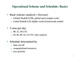
Operational Scheme and Schedule: Basics • Basic scheme (analysis + forecast) • Global-Modell (GME, global and synoptic-scale) • Lokal Modell (LM, highly resolved mesoscale model) • 3 runs per day • 00, 12, 18 UTC • 03, 06, 09, 15, 21 UTC only analysis • Schedule determined by • data cut-off • computational resources • user priority
Boundary values and forecast range • forecast range of LM: 48h • every hour LM gets new boundary data from GME • smooth transition within 8 grid points • continous data assimilation • forecast range of GME • 00, 12 UTC: 174h • 18 UTC: 48h
Schedule of GME/LM-runs (relative to starting time) • +2h 06min start of GME-analysis • +2h 23 min start of LM-analysis • +2h 30 min start of GME-forecast • +2h 34 min start of LM-forecast • +3h 45 min 48h-LM-forecast available • +4h 30 min 174h-GME-forecast available • Postprocessing- • Graphic-files: 5 min • local forecast parameters: 15 min • Availability of final products about 5 hours after starting time
Basic postprocessing • Interpolation between model levels and pressure levels • model level (34m): Typical vertical profiles (depending on stability, e.g) • T 2m • wind 10m • LM-model-levels 26 and 27 for 850-hPa-level, e.g • Reduction of model surface pressure to mean sea level • base: adiabatic gradient • in the case of mountainous areas (e.g. Greenland) • reduced amount of vertical temperature gradient • however, often too high surface pressure values
Postprocessing (further steps) • Automatic weather interpretation • for all fields and local products: describing model weather output of GME and LM • Generation of graphical and alphanumerical products • general analysis and forecast fields • MPEG-files (TriVis) with animations of • cloud development • precipication • wind • temperature • local model output as meteograms and local soundings • local direct model output as alphanumerical information • local output through Kalman, Model Output Statistics and Perfect Prog
Postprocessing (Cross Sections) • Time series of preselected cross-sections of relevant parameters • cloudiness • wind • temperature
Postprocessing (followed-up-models) • Followed-up models (based upon GME-/LM-output) • sea state models • water level (e.g. tides) • waves • trajectory model • pollution (e.g.) • winter road maintenance • SWIS (1-D-model for road surface temperature and road condition) • agro- and biometeorological models • fungus disease • ultraviolett irradiation • test: 1-D-model for fog and low clouds
Computer-system: NWP-runs, IBM • distributed memory massively parrallel processors • application units: 1920 • different model areas are related to different processors • communication between these areas is performed • COS4: 448, COS5: 1472 processor units • memory: 1240 GByte • disk capacity: 7562 GByte • peak performance of each processor unit: 2.4 GFlop/s • „beat frequency“: 375 MHz • each „beat“ : e.g. 8 floating point operations (by considering more bits)!
Computer-system: data storage, communication (I) • 2 IBM p690, each • 32 processors • 128 GB memory • 864 GB disk capacity • tasks (e.g.) • developments, tests • routine jobs (decoding of observations, production of graphics, etc) • data handling • Storage server (e.g., test results) • 3 x 13.5 TByte
Computer-system: data storage, communication (II) • data amount • 174h-GME-run: 40 GByte • 48h-LM-run: 5 GByte • totaly NWP-production > 120 Gbyte per day (follow-up models inclusive ) • Archive (SGI O200) • 24 processors • 24 GB memory • 853 GB disc capacity • archiving of data on cassettes (600 TByte)