Molecular phylogenetics continued…

1. Molecular phylogenetics continued…

2. Outline 1. Models of evolution 2. Phylogenetic tree reconstruction methods: -- distance based methods -- maximum parsimony (MP) -- maximum likelihood (ML) 3. Bootstrapping: evaluating the significance of a tree

3. The simplest model of evolution: pairwise distance The simplest approach to measuring distances between sequences is to align pairs of sequences, and then to count the number of differences. The degree of divergence is called the p-distance. For an alignment of length N with n sites at which there are differences, the degree of divergence D is: D = n / N Consider an alignment where 3/60 aligned residues differ. The p-distance is 3/60 = 0.05.

4. Common assumptions of simple evolutionary models • Simple models of the evolutionary process make several incorrect assumptions: • equal base or amino acid substitution rates • an equal frequency of all bases or amino acids • an equal evolutionary rate at all sites of an alignment • 4) independent evolution between sites of an alignment. Observations of DNA/protein alignments demonstrates these assumptions are often not met in nature. Therefore much more realistic models of DNA/protein evolution have been devised (more on this to follow).

5. Evolutionary models: The Poisson distance correction -- A simple correction of the p-distance can be derived by assuming the probability of mutation at a site follows a Poisson distribution (with a uniform mutation rate) -- Correction takes account of multiple mutations at the same site

6. Evolutionary models: The Poisson distance correction -- A simple correction of the p-distance can be derived by assuming the probability of mutation at a site follows a Poisson distribution (with a uniform mutation rate) -- Correction takes account of multiple mutations at the same site Poisson corrected distance: dp = -ln(1-p) -- The corrected distance starts to deviate noticeably from the p-distance for p > 0.25 Assumption: equal rate of mutation at all sites Figure 8.1

7. Evolutionary models: the Gamma distance correction -- The Gamma distance correction takes account of mutation rate variation at different sites -- A Gamma distribution (Γ) can effectively model realistic variation in mutation rates

8. Evolutionary models: the Gamma distance correction -- The Gamma distance correction takes account of mutation rate variation at different sites -- A Gamma distribution (Γ) can effectively model realistic variation in mutation rates DΓ = a[(1-p)-1/a– 1] -- The parameter a determines the rate variation -- Values of a estimated from real protein sequence data vary between 0.2 (high variation) and 3.5 (lower variation) Figure 8.2

9. Evolutionary models p-distance, Poisson model, Gamma distance correction: These mutation models do not include any information relating to the chemical nature of the sequences, which means they can be applied to both nucleotide and protein sequences. So, it follows that there are a whole series of more complex evolutionary models specific for nucleotide sequence or protein sequence evolution

10. Jukes and Cantor (JC) one-parameter model of nucleotide substitution: all substitutions occur with equal probability a A G Substitution rate matrix A C G T -3α α α α α -3α α α α α -3α α α α α -3α a A C G T a a a T C a P. 271

11. Kimura two-parameter model (K2P) of nucleotide substitutions: the probability of transitions and transversion occurring are different a A G Substitution rate matrix A C G T -2β-α β α β β -2β-α α α α β -2β-α β β α α -2β-α b A C G T b b b T C a P. 272

12. Incorporation of unequal base frequencies HKY85 substitution rate matrix: this is a K2P model, but rate matrix has been modified to account for differences in base composition (πA:πC:πG:πT) A C G T (-2β-α)πA βπC απG βπT βπA (-2β-α)πC απG απT απA βπC (-2β-α)πG βπT βπA απC απG (-2β-α)πT A C G T P. 273

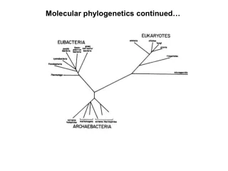
13. Different models of molecular evolution (nucleotides) Table 7.2

14. Evolutionary models: amino acid substitution matrices There are empirically based models of amino acid substitution, which consist of a 20 x 20 rate matrix that estimates the probabilities for each amino acid being replaced by each alternative amino acid. The Jones-Taylor-Thornton model (JTT) is the same as the Dayhoff models but based on a more up to date substitution matrix constructed from a larger database of sequence The PMB model is derived from the BLOCKS database of conserved protein motifs and is therefore related to BLOSUM

15. Common assumptions of simple evolutionary models • Simple models of the evolutionary process make several incorrect assumptions: • equal base or amino acid substitution rates • an equal frequency of all bases or amino acids • an equal evolutionary rate at all sites of an alignment • 4) independent evolution between sites of an alignment. Observations of DNA/protein alignments demonstrates these assumptions are often not met in nature. Therefore much more realistic models of DNA/protein evolution have been devised

16. Common assumptions of simple evolutionary models • Simple models of the evolutionary process make several incorrect assumptions: • equal base or amino acid substitution rates  solution: use a more complex substitution matrix • an equal frequency of all bases or amino acids  solution: estimate from sequence alignment data • an equal evolutionary rate at all sites of an alignment  solution: model among site rate variation (ASRV) with a Gamma distribution • 4) independent evolution between sites of an alignment  solution: yikes! No easy solution here…

17. How to select an appropriate evolutionary model: While it is easy to identify models that are formally more realistic, these are not necessarily more effective in representing the real data (i.e. the MSA) Figure 7.18

18. How to select an appropriate evolutionary model: While it is easy to identify models that are formally more realistic, these are not necessarily more effective in representing the real data (i.e. the MSA) Figure 7.18

19. How to select an appropriate evolutionary model: While it is easy to identify models that are formally more realistic, these are not necessarily more effective in representing the real data (i.e. the MSA) Example of model selection Akaike information criterion (AIC): measures the support in the data for a given model. The model with the smallest AIC value is regarded as the most suitable Table 7.3

20. Outline 1. Models of evolution 2. Phylogenetic tree reconstruction methods: -- distance based methods -- maximum parsimony (MP) -- maximum likelihood (ML) 3. Bootstrapping: evaluating the significance of a tree

21. Phylogenetic tree reconstruction Phylogenetic inference is an hypothesis-generating procedure, where an inferred tree represents the “best hypothesis” of evolutionary relationships based on the limited information contained in molecular sequence data and the assumptions of the phylogenetic reconstruction method. Of the many possible evolutionary histories that could produce the observed differences between homologous sequences, we must have some method for choosing one or more best trees from all possible trees.

22. Tree reconstruction methods Algorithmic methodsfollow a fixed series of procedures (an algorithm) to derive a tree from the data. - computationally fast - how well the tree fits the data relative to an alternative tree is unknown. - e.g. UPGMA or neighbor-joining methods

23. Tree reconstruction methods Algorithmic methodsfollow a fixed series of procedures (an algorithm) to derive a tree from the data. - computationally fast - how well the tree fits the data relative to an alternative tree is unknown. - e.g. UPGMA or neighbor-joining methods Optimality criterionmethodsdefine a criterion for comparing trees and then finds the tree that maximizes/minimizes the criterion. - can define how good or bad any one tree is compared to other possibilities - e.g. maximum parsimony and maximum likelihood methods

24. Outline 1. Models of evolution 2. Phylogenetic tree reconstruction methods: -- distance based methods -- maximum parsimony (MP) -- maximum likelihood (ML) 3. Bootstrapping: evaluating the significance of a tree

25. Distance matrix methods • Phylogenetic inference by distance matrix methods involves two sequential steps: • the evolutionary distances (i.e. number of substitutions) between all taxa in an alignment is estimated based on a model of evolution. • the results are tabulated in a distance matrix and one of a variety of approaches is used to reconstruct a phylogenetic tree from the pairwise distance values.

26. The general flow of a distance matrix method for phylogenetic inference Species A Species B Species C Species D Species E Species A Species B Species C Species D Species A Species B Species C Species D Species E Species D Species C Species B Species E Species A

27. Inferring a tree from a distance matrix The simplest algorithm is Unweighted pair-group method with arithmetic mean (UPGMA). UPGMA uses a sequential clustering algorithm to group taxa in order of decreasing similarity. Ultrametric tree The details of this algorithm are presented in Chapter 8 (p 278-279)

28. Assumptions of UPGMA UPGMA makes the assumption that there is a linear relationship between evolutionary distance and divergence time, or, in other words, that the rate of evolution is equal and constant among taxa(i.e. ultrametric or clock-like). This assumption is rarely, if ever, met and therefore it is advised that UPGMA not be used to infer a best tree. There are many other superior methods for tree reconstruction that are as easy to implement and are computationally fast.

29. The neighbor joining (NJ) method NJ does not assume all sequences have the same constant rate of evolution The basis of the method lies in the concept of minimum evolution, specifically that the tree with the shortest total branch length is the best tree The first steps of NJ; start with a star tree, identify the first pair of nearest neighbors… full details on p 282- 285 NJ is a star decomposition algorithm that attempts to minimize the overall branch length of the tree. Figure 8.6

30. Neighbor joining method Modified versions of the original neighbor-joining method such as BioNJ and Weighbor have been formulated and they tend to outperform the original neighbor-joining algorithm. Because of fast run times neighbor-joining is particularly useful for large studies or bootstrap resampling studies that require analysis of multiple datasets (e.g. Bootstrap Analysis).

31. Outline 1. Models of evolution 2. Phylogenetic tree reconstruction methods: -- distance based methods -- maximum parsimony (MP) -- maximum likelihood (ML) 3. Bootstrapping: evaluating the significance of a tree

32. Parsimony methods Parsimony methods are based on the concept that the best hypothesis is the one that requires the least amount of evolutionary changes. Objective: to find the tree (i.e. hypothesis) that requires the minimum number of substitutions to explain the observed/inferred difference between sequences. Maximum parsimony (MP) is thus an optimality-criterion method in which the criterion (i.e. number of substitutions) is to be minimized. The tree that minimizes the number of substitutions required to explain the data is called the maximum parsimony tree.

33. There are only 3 possible trees with 4 taxa A C A C D D B B A D A B B C C D Which two trees are the same?

34. Parsimony methods Parsimony begins with the classification of sites as either informative or uninformative. A site is considered informative if it favors a subset of trees over all possible trees. Site 1 is uninformative because the character states are all identical

35. Parsimony methods Parsimony begins with the classification of sites as either informative or uninformative. A site is considered informative if it favors a subset of trees over all possible trees. Site 2 is uninformative because there are two mutations required for all possible trees

36. Site 2 is uninformative (2 substitutions in all trees)

37. Site 3 is informative and tree 1 is most parsimonious

38. Site 4 is informative and tree 2 is most parsimonious

39. Tree 2 is the maximum parsimony tree Site 5 is informative and tree 2 is most parsimonious

40. Searching through the “forest” for the “best tree” As the number of taxa becomes large (10+), the number of possible trees becomes enormous and searching this “tree space” for the optimal tree can become computationally impossible. Procedures exist for reducing the search time (e.g. heuristic search)

41. Searching tree space Heuristic tree searches seek the optimal tree though the use of iterative trial and error processes, which examine a subset of all possible trees Some common branch swapping algorithms: Nearest neighbor interchange (NNI) a branch swapping method that results in local rearrangements of a tree. Subtree pruning and regrafting (SPR), all possible subtrees are “pruned” from the reference tree and then “regrafted” at an alternative location.

42. Problems with parsimony Correct phylogeny True convergent evolution Incorrect reconstruction This inconsistency in parsimony clusters long branches together and is termed “long branch attraction”. It can be a problem in all phylogenetic methods.

43. Outline 1. Models of evolution 2. Phylogenetic tree reconstruction methods: -- distance based methods -- maximum parsimony (MP) -- maximum likelihood (ML) 3. Bootstrapping: evaluating the significance of a tree

44. Maximum likelihood methods Maximum likelihood is an optimality based method, which evaluates a hypothesized tree in terms of the probability that it would lead to the observed sequence data under a proposed model of evolution. ML methods are among the most accurate at inferring phylogenetic trees, but also some of the most time consuming methods to run The principle of maximum likelihood is to find the tree that maximizes the likelihood of observing the data.

45. Maximum likelihood methods Maximum likelihood is an optimality based method, which evaluates a hypothesized tree in terms of the probability that it would lead to the observed sequence data under a proposed model of evolution. The principle of maximum likelihood is to find the tree that maximizes the likelihood of observing the data. Data Hypothesis

46. A very brief overview of the maximum likelihood method 1) Calculate the likelihood (L) of each site given the tree

47. A very brief overview of the maximum likelihood method 1) Calculate the likelihood (L) of each site given the tree 2) Sum the ln (L) to get the likelihood of the whole alignment This calculation must be performed for each tree during a heuristic search

48. Outline 1. Models of evolution 2. Phylogenetic tree reconstruction methods: -- distance based methods -- maximum parsimony (MP) -- maximum likelihood (ML) 3. Bootstrapping: evaluating the significance of a tree

49. Error associated with inferred trees Random erroris the deviation from the true tree, because there is a limited length of sequence data. Random error will therefore tend to decrease with an increasing length of data, as the stochastic variation associated with small sample size becomes less. Systematic erroris the deviation from the true tree due to incorrect assumptions in the method or model used for phylogenetic inference. Systematic error will introduce a bias that may support the wrong tree and, unlike random error, the addition of more data will tend to increase support for the incorrect tree.

50. Evaluating trees: bootstrapping Bootstrapping is a commonly used approach to measuring the robustness of a tree topology. Given a branching order, how consistently does A phylogenetic method find that branching order in a randomly permuted version of the original data set? IMPORTANT: Bootstrapping allows an assessment of random error only, not systematic error due to inaccurate assumptions in an evolutionary model.