Download
1 / 49
490 likes | 513 Vues
This paper discusses the range of possible surface reconstructions from gradient fields, including methods to handle noise and outliers while preserving features. Various approaches such as least squares, Poisson solvers, and transformation of gradients are explored. The paper also introduces different techniques for integrability and the use of basis functions. The limitations of least squares approaches are discussed, and alternative methods that offer more robust and feature-preserving solutions are presented.

E N D
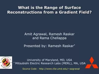
What is the Range of Surface Reconstructions from a Gradient Field? Amit Agrawal, Ramesh Raskar and Rama Chellappa Presented by: Ramesh Raskar* University of Maryland, MD, USA * Mitsubishi Electric Research Labs (MERL), MA, USA Source Code: http://www.cfar.umd.edu/~aagrawal
Overview • Goal: Reconstruct height field from a gradient field • Challenges • Handle noise and outliers • Tradeoff: Preserve features or smooth • Provide knobs for control ? X Gradient Y Gradient Height Field
Choices of Reconstructions Noisy Gradients Height Field Least Sq Solution Robust Solution MSE = 10.81 MSE = 2.26
A Range of Reconstructions 1. Generalized Solution Isotropic Anisotropic Poisson Solver Alpha-Surface M-estimator, Regularization Diffusion Continuous weights Binary weights Affine Transformation Scaling 2. Linear transformation of gradient vectors
Source of Gradients: Image Manipulation 2D Integration Grad X New Grad X Gradient Processing New Grad Y Grad Y Forward Difference Modified Gradients(Non-integrableGradients) Image
X Gradient Y Gradient Source of Gradients: Photometric Stereo Mozart Images under varying illumination (Non-integrable Gradients) 2D Integration Robust Solution MSE=2339.2 MSE=373.72
Gradient Field Integration • Photometric Stereo • Phase unwrapping, Mesh smoothing • Retinex (Horn’74) • HDR compression (Fattal’02) • Poisson image editing (Perez’04) • Poisson matting (Sun’04) • Image fusion (Raskar’04), Multi-flash Camera (Raskar’04) • Image Stitching (Levin’04) • Flash/No-flash (Agrawal’05) • ..
Space of Solutions Non-Integrable Gradient Field Robust solutions Residual Field Least Squares solution Subspace of Integrable Gradient Fields Space of All Gradient Fields
Example Application: Photometric Stereo • How to obtain heights from gradient field? • Preserve features during integration • Handle noise and outliers Z p q ? X Gradient Y Gradient Height Field
Integrability • Gradient field of solution Z should be integrable • Curl(Zx,Zy) (loop integrals) should be zero • Noisy estimated gradient field is non-integrable • Curl(p,q) ≠ 0
Common approaches to handle Integrability • Least Square: • Minimize error between • Estimated gradients (p,q) and Gradients of solution Z • [Horn et al. IJCV’90], [Simchony et al. PAMI’90] • Solution: Poisson equation Divergence Laplacian
Integrability: Reconstruction using Basis Functions • Project non-integrable gradients onto basis functions • Fourier: Frankot-Chellappa (PAMI’88) • Cosine: Georghiades (PAMI’01) • Redundant basis: Kovesi (ICCV’05)
Limitations of Least Squares Approaches • Lack of robustness • Smooth solution rather than feature preserving • Cannot handle outliers Height Field Least Sq Solution Robust Solution MSE = 10.81 MSE = 2.26
Key Ideas • All gradients are not required for integration • Replace gradients by functions of gradients
Approach • Transform input and output gradients • Poisson equation Unknown (Output) Gradients of Height Field Z Estimated(Input) Gradients
Approach • Transform input and output gradients • Poisson equation • New Generalized Equation Functions of Output Gradients Functions of Input Gradients
Approach • Transform input and output gradients • Poisson equation • New Generalized Equation • Knobs for control: functions f1, f2, f3, f4 fi
Least Squares Poisson Solution Isotropic Anisotropic Alpha-Surface M-estimator, Regularization Diffusion Poisson Solver Continuous weights Binary weights Affine Transformation Scaling No Change f1(Zx,Zy) f2(Zx,Zy) f3(p,q) f4(p,q) Poisson solver Zx Zy p q
A Range of Solutions by Transforming Gradients Anisotropic Isotropic Poisson Solver Alpha-Surface M-estimator, Regularization Diffusion Continuous weights Binary weights Affine Transformation Scaling fi Linear Transformation of Gradient Vectors using fi
A Range of Solutions by Transforming Gradients Anisotropic Isotropic Poisson Solver Alpha-Surface M-estimator, Regularization Diffusion Continuous weights Binary weights Affine Transformation Scaling fi f1(Zx,Zy) f2(Zx,Zy) f3(p,q) f4(p,q) Poisson solver Zx Zy p q 1. -surface bxZx byZy bxp byq 2. M-estimators wxZx wyZy wxp wyq 3. Regularization wxZx wyZy p q 4. Diffusion d11Zx+d12Zy d12Zx+d22Zy d11p+d12q d12p+d22q
Anisotropic Isotropic Poisson Solver Alpha-Surface M-estimator, Regularization Diffusion Continuous weights Binary weights Affine Transformation Scaling A Range of Solutions 1. Robust Estimation by ignoring outliers in gradients
1. -Surface: Binary Weights • Classifying gradients as inliers/outliers • Based on tolerance • Graph Analogy • 2D grid as a planar graph • Nodes correspond to height values • Edges correspond to gradient values • Given edges compute nodes • [Agrawal et al ICCV 2005]
All Gradients are not required • Minimal set is the spanning tree of the graph • All nodes can be reached via spanning tree • N2 -1 edges in spanning tree for N2 nodes • Dimensionality of gradient field ~= 2N2 • Dimensionality of solution space = N2 - 1
- Surface • Start with minimum spanning tree • Minimal set of (N2-1) edges • Iterate • Integrate height field using (inlier) edges • Compute gradient edges of the solution • Find inlier edges using tolerance
Tolerance d d< d
Choice of = 0Minimum Spanning TreeUnique SolutionRobust to outliers >>Overconstrained: All GradientsLeast Squares SolutionSmooth
Anisotropic Isotropic Poisson Solver Alpha-Surface M-estimator, Regularization Diffusion Continuous weights Binary weights Affine Transformation Scaling A Range of Solutions 2. Robust Estimation by weighting gradients
2. Continuous Weights Solution • M-estimators • Formulated as iterative re-weighted least squares • wx, wy are weights applied to gradients Least squares Huber Influence function
3. Regularization • Add edge-preserving term using function Ф • Solved iteratively • Estimate weights wx, wy using Z • Update Z using weights • We use
Anisotropic Isotropic Poisson Solver Alpha-Surface M-estimator, Regularization Diffusion Continuous weights Binary weights AffineTransformation Scaling A Range of Solutions 4. Robust Estimation by affine transformation of gradients
4. Affine transformation of Gradient Field • General Transform of Gradients Vectors • Matrix D2x2 is a field of tensors • Estimated using the input gradient field (p,q) • Similar to edge-preserving diffusion tensor • Image Restoration [Weickert’96]
4. Affine transformation of Gradient Field • Transformed gradient vectors • Non-iterative, sparse linear system f1(Zx,Zy) f2(Zx,Zy) f3(p,q) f4(p,q) d11Zx+d12Zy d12Zx+d22Zy d11p+d12q d12p+d22q
Mozart: Sharp Features MSE=219.72 MSE=2339.2 MSE=1316.6 MSE=359.12 MSE=806.85 MSE=373.72
Vase: Smooth Object MSE=294.5 MSE=239.6 MSE=22.2 MSE=164.98 MSE=15.14 MSE=2.78
Isotropic Anisotropic Poisson Solver Alpha-Surface M-estimator, Regularization Diffusion Continuous weights Binary weights Affine Transformation Scaling Generalized Solution using Gradient Vector Transformation Ground Truth Least Squares Feature Preserving
Isotropic Anisotropic Poisson Solver Alpha-Surface M-estimator, Regularization Diffusion Continuous weights Binary weights Affine Transformation Scaling Reconstruction from Gradients • Gradient Field integration as robust estimation • Generalized equation • Isotropic case: Least-square solution • Anisotropic transforms: Range of feature preserving solutions • Knobs for meaningful control • Future Directions • Automatic choice of anisotropic function • Nth order error functions • Using control/seed points information Source Code: http://www.cfar.umd.edu/~aagrawal
H W Space of All solutions • For a H*W grid, all solutions lie in a subspace of dimension HW-1 • Equations • W-1 loops for each row, H-1 loops for each column • Total number of independent equations • N = (H-1)(W-1) = HW – H –W + 1 • Unknowns • W-1 x gradients in H rows, H-1 y gradients in W columns • Total unknowns • M = (W-1)*H + (H-1)*W = 2HW – H - W
Linear System • Stack all equation to form Ax = b • b contains negative of the curl values • x contains all the residual gradient values (pε,qε) • A is a sparse matrix with each row having 4 non-zero elements • Under-constrained system. A has null space of dimension M-N = H*W-1 • xp = particular solution Axp = b • Xh = homogeneous solution Axh= 0
p q Images X Gradient Y Gradient Example Application: Photometric Stereo • Multiple images, varying illumination • Obtain surface gradient field from images • Lambertian reflectance model
Mozart: Sharp Features MSE=219.72 MSE=2339.2 MSE=1316.6 MSE=359.12 MSE=806.85 MSE=373.72
Vase: Smooth Object MSE=294.5 MSE=239.6 MSE=22.2 MSE=164.98 MSE=15.14 MSE=2.78
Choice of = 0Minimum Spanning TreeUnique SolutionRobust to outliers >>Overconstrained: All GradientsLeast Squares SolutionSmooth Toy Example
Choosing spanning tree • Assign weights to edges based on gradients • Find minimum spanning tree (MST) • Compute based on variance
Face Input Images Estimated Heights with -tolerance
3. Regularization • Add edge-preserving term using function Ф • Solved iteratively • Estimate weights wx, wy using Z • Update Z using weights • We use