Concept of Probability
Probability theory is a natural language for describing real-world phenomena, developed over centuries by key figures like Pascal and Laplace. This complex concept reflects the uncertainty of events based on information available. To calculate probabilities, one must understand sample spaces and apply rules such as addition and multiplication. Through examples like rolling dice or predicting birthdates, probabilities can be calculated effectively, enhancing decision-making in various scenarios.

Concept of Probability
E N D
Presentation Transcript
Concept of Probability AS3105 Astrophysical Processes 1 Dhani Herdiwijaya
Probability in Everyday Life • Rain fall • Traffic jam • Across the street • Catastrophic meteoroid • airplane travel. Is it safe to fly? Laplace (1819) Probability theory is nothing but common sense reduced to calculation Maxwell (1850) The true logic of this world is the calculus of probabilities . . . That is, probability is a natural language for describing real world phenomena A mathematical formulation of games of chance began in the middle of the 17th century. Some of the important contributors over the following 150 years include Pascal, Fermat, Descartes, Leibnitz, Newton, Bernoulli, and Laplace
Development it is remarkable that the theory of probability took so long to develop. An understanding of probability is elusive due in part to the fact that the probably depends on the status of the information that we have (a fact well known to poker players). Although the rules of probability are defined by simple mathematical rules, an understanding of probability is greatly aided by experience with real data and concrete problems.
Probability To calculate the probability of a particular outcome, count the number of all possible results. Then count the number that give the desired outcome. The probability of the desired outcome is equal to the number that gives the desired outcome divided by the total number of outcomes. Hence, 1/6 for one die.
Rules of Probability In 1933 the Russian mathematician A. N. Kolmogorov formulated a complete set of axioms for the mathematical definition of probability. For each event i, we assign a probability P(i) that satisfies the conditions P (i) ≥ 0 P (i) = 0 means that the event cannot occur P (i) = 1 means that the event must occur
The normalization condition says that the sum of the probabilities of all possible mutually exclusive outcomes is unity Example. Let x be the number of points on the face of a die. What is the sample space of x? Solution. The sample space or set of possible events is xi = {1, 2, 3, 4, 5, 6}. These six outcomes are mutually exclusive. There are many different interpretations of probability because any interpretation that satisfies the rules of probability may be regarded as a kind of probability. An interpretation of probability that is relatively easy to understand is based on symmetry.
Addition rule For an actual die, we can estimate the probability a posteriori, that is, by the observation of the outcome of many throws. Suppose that we know that the probability of rolling any face of a die in one throw is equal to 1/6, and we want to find the probability of finding face 3 or face 6 in one throw. the probability of the outcome, i or j , where i is distinct from j P (i or j ) = P (i) + P (j ). (addition rule) The above relation is generalizable to more than two events. An important consequence is that if P (i) is the probability of event i, then the probability of event i not occurring is 1 − P (i).
Combining Probabilities • If a given outcome can be reached in two (or more) mutually exclusive ways whose probabilities are pA and pB, then the probability of that outcome is: pA + pB. • This is the probability of having eitherA or B.
Example • Paint two faces of a die red. When the die is thrown, what is the probability of a red face coming up?
Example: What is the probability of throwing a three or a six with one throw of a die? Solution. The probability that the face exhibits either 3 or 6 is 1/6 + 1/6 = 1/3 Example: What is the probability of not throwing a six with one throw of die? Solution. The answer is the probability of either “1 or 2 or 3 or 4 or 5.” The addition rule gives that the probability P (not six) is P (not six) = P (1) + P (2) + P (3) + P (4) + P (5) = 1 − P (6) = 5/6 the sum of the probabilities for all outcomes sums to unity. It is very useful to take advantage of this property when solving many probability problems.
Multiplication rule • Another simple rule is for the probability of the joint occurrence of independent events. These events might be the probability of throwing a 3 on one die and the probability of throwing a 4 on a second die. If two events are independent, then the probability of both events occurring is the product of their probabilities P (i and j ) = P (i) P (j ) (multiplication rule) • Events are independent if the occurrence of one event does not change the probability for the occurrence of the other.
Combining Probabilities • If a given outcome represents the combination of two independent events, whose individual probabilities are pA and pB, then the probability of that outcome is: pA × pB. • This is the probability of having bothA and B.
Example • Throw two normal dice. What is the probability of two sixes coming up?
Example: Consider the probability that a person chosen at random is female and was born on September 6. We can reasonably assume equal likelihood of birthdays for all days of the year, and it is correct to conclude that this probability is ½ x 1/365 Being a woman and being born on September 6 are independent events.
Example. What is the probability of throwing an even number with one throw of a die? Solution. We can use the addition rule to find that P (even) = P (2) + P (4) + P (6) = 1/6 + 1/6 +1/6 = ½ • Example. What is the probability of the same face appearing on two successive throws of a die? Solution. We know that the probability of any specific combination of outcomes, for example, (1,1), (2,2), . . . (6,6) is 1/6 x 1/6 = 1/36 P (same face) = P (1, 1) + P (2, 2) + . . . + P (6, 6) = 6 × 1/36 = 1/6
Solution. We have already established that P (6) = 1/6 and P (not 6) = 5/6. In two throws, there are four possible outcomes (6, 6), (6, not 6), (not 6, 6), (not 6, not 6) with the probabilities P (6, 6) = 1/6 x 1/6 = 1/36 P (6, not 6) = P (not 6, 6) = 1/6 x 5/6 = 5/36 P (not 6, not 6) = 5/6 x 5/6 = 25/36 All outcomes except the last have at least one six. Hence, the probability of obtaining at least one six is P (at least one 6) = P (6, 6) + P (6, not 6) + P (not 6, 6) = 1/36 + 5/36 + 5/36 = 11/36 A more direct way of obtaining this result is to use the normalization condition. That is, P (at least one six) = 1 − P (not 6, not 6) = 1 − (5/6)2 = 1 - 25/36 = 11/36 ~ 0.305… • Example. What is the probability that in two throws of a die at least one six appears?
Example. What is the probability of obtaining at least one six in four throws of a die? Solution. We know that in one throw of a die, there are two outcomes with P (6) = 1/6 and P (not 6) = 5/6 . Hence, in four throws of a die there are sixteen possible outcomes, only one of which has no six. That is, in the fifteen mutually exclusive outcomes, there is at least one six. We can use the multiplication rule to find that P (not 6, not 6, not 6, not 6) = P (not 6)4 = (5/6)4 and hence P (at least one six) = 1 − P (not 6, not 6, not 6, not 6) = 1 - (5/6)4 = 671/1296 ~ 0.517
Complications p is the probability of success. (1/6 for one die) q is the probability of failure. (5/6 for one die) • p + q = 1, or q = 1 – p When two dice are thrown, what is the probability of getting only one six?
Complications • Probability of the six on the first die and not the second is: • Probability of the six on the second die and not the first is the same, so:
Simplification • Probability of no sixes coming up is: • The sum of all three probabilities is: • p(2) + p(1) + p(0) = 1
Simplification • p(2) + p(1) + p(0) = 1 • p² + 2pq + q² =1 • (p + q)² = 1 The exponent is the number of dice (or tries). • Is this general?
Three Dice • (p + q)³ = 1 • p³ + 3p²q + 3pq² + q³ = 1 • p(3) + p(2) + p(1) + p(0) = 1 • It works! It must be general! (p + q)N = 1
Renormalization Suppose we know that P (i) is proportional to f (i), where f (i) is a known function. To obtain the normalized probabilities, we divide each function f (i) by the sum of all the unnormalized probabilities. That is, if P (i) α f (i), and Z = ∑ f (i), then P (i) = f (i)/Z . This procedure is called normalization.
Example. Suppose that in a given class it is three times as likely to receive a C as an A, twice as likely to obtain a B as an A, one-fourth as likely to be assigned a D as an A, and nobody fails the class. What are the probabilities of getting each grade? Solution. We first assign the unnormalized probability of receiving an A as f (A) = 1. Then f (B ) = 2, f (C ) = 3, and f (D) = 0.25. Then Z = ∑ f (i) = 1 + 2 + 3 + 0.25 = 6.25. Hence, P (A) = f (A)/Z = 1/6.25 = 0.16, P (B ) = 2/6.25 = 0.32, P (C ) = 3/6.25 = 0.48, and P (D) = 0.25/6.25 = 0.04.
Meaning of Probability • How can we assign the probabilities of the various events? If we say that event E1 is more probable than event E2 (P (E1 ) > P (E2 )), we mean that E1 is more likely to occur than E2 . This statement of our intuitive understanding of probability illustrates that probability is a way of classifying the plausibility of events under conditions of uncertainty. Probability is related to our degree of belief in the occurrence of an event. • Probability assessments depend on who does the evaluation and the status of the information the evaluator has at the moment of the assessment. We always evaluate the conditional probability, that is, the probability of an event E given the information I , P (E | I ). Consequently, several people can have simultaneously different degrees of belief about the same event, as is well known to investors in the stock market.
If rational people have access to the same information, they should come to the same conclusion about the probability of an event. The idea of a coherent bet forces us to make probability assessments that correspond to our belief in the occurrence of an event. Probability assessments should be kept separate from decision issues. Decisions depend not only on the probability of the event, but also on the subjective importance of say, a given amount of money
Probability and Knowledge • Probability as a measure of the degree of belief in the occurrence of an outcome implies that probability depends on our prior knowledge, because belief depends on prior knowledge. • Probability depends on what knowledge we bring to the problem. If we have no knowledge other than the possible outcomes, then the best estimate is to assume equal probability for all events. However, this assumption is not a definition, but an example of belief. As an example of the importance of prior knowledge, consider the following problem.
Large numbers We can estimate probabilities empirically by sampling, that is, by making repeated measurements of the outcome of independent events. Intuitively we believe that if we perform more and more measurements, the calculated average will approach the exact mean of the quantity of interest. We should use computer to generate random number. The applet/application at <stp.clarku.edu/simulations/cointoss> to simulate multiple tosses of a single coin This idea is called the law of large numbers.
Mean Value • Consider the probability distribution P (1), P (2), . . . P (n) for the n possible values of the variable x. In many cases it is more convenient to describe the distribution of the possible values of x in a less detailed way. The most familiar way is to specify the average or mean value of x, which we will denote as <x>. The definition of the mean value of <x> is <x> ≡ x1 P (1) + x2 P (2) + . . . + xnP (n) where P (i) is the probability of xi . If f (x) is a function of x, then the mean value of f (x) is defined by
Example:A certain $50 or $100 if you flip a coin and get a head and $0 if you get a tail. The mean value for the second choice is mean value = ∑ Pi × (value of i), where the sum is over the possible outcomes and Pi is the probability of outcome i. In this case the mean value is 1/2 × $100 + 1/2 × $0 = $50. We see that the two choices have the same mean value. (Most people prefer the first choice because the outcome is “certain.”)
If f (x) and g(x) are any two functions of x, then <f (x) + g(x)> = ∑ [f (xi) + g(xi )] P (i) = ∑ f (xi) P (i) + ∑ g(xi) P (i) or <f (x) + g (x)> = <f (x)> + <g (x)> if c is a constant, then <c f (x)> = c <f (x)> In general, we can define the mth moment of the probability distribution P as <xm> ≡ ∑ xim P (i) where we have let f (x) = xm . The mean of x is the first moment of the probability distribution
The mean value of x is a measure of the central value of x about which the various values of xi are distributed. If we measure x from its mean, we have that Δx ≡ x − <x> <Δx> = <(x − <x>)> = <x> − <x> = 0 That is, the average value of the deviation of x from its mean vanishes If only one outcome j were possible, we would have P (i) = 1 for i = j and zero otherwise, that is, the probability distribution would have zero width. In general, there is more than one outcome and a possible measure of the width of the probability distribution is given by <Δx2> ≡ <(x − <x>)2> The quantity <Δx2> is known as the dispersion or variance and its square root is called the standard deviation. It is easy to see that the larger the spread of values of x about <x>, the larger the variance.
The use of the square of x − <x> ensures that the contribution of x values that are smaller and larger than <x> enter with the same sign. A useful form for the variance can be found by noting that <(x − <x>)2> = <(x2 − 2x<x> + <x>2)> = <x2> - 2 <x><x> + <x>2 = <x2> - <x>2 Because <Δx2> is always nonnegative, it follows that <x2> ≥ <x>2 it is useful to interpret the width of the probability distribution in terms of the standard deviation σ, which is defined as the square root of the variance. The standard deviation of the probability distribution P (x) is given by σx = square (<Δx2>) = square (<x2> - <x>2)
Example: Find the mean value <x>, the variance <Δx2>, and the standard deviation σx for the value of a single throw of a die. Solution. Because P (i) = 1/6 for i = 1, . . . , 6, we have that <x> = 1/6 (1+2+3+4+5+6) = 7/2 <x2> = 1/6 (1 + 4 + 9 + 25 + 36) = 46/3 (<Δx2>) = <x2> - <x>2 = 46/3 – 49/4 = 37/12 ~ 3.08 σx = square (3.08) ~ 1.76
Home work There is an one-dimensional lattice constant a as shown in Fig. 1. An atom transit from a site to a nearest-neighbor site every r second. The probability of transiting to the right and left are p and q = 1 – p, respectively. (a) Calculate the average position <x> of the atom at the time t = Nτ, where N >> 1 (b) Calculate the mean square value <(x - <x>)2> at the time t
Ensemble Another way of estimating the probability is to perform a single measurement on many copies or replicas of the system of interest. For example, instead of flipping a single coin 100 times in succession, we collect 100 coins and flip all of them at the same time. The fraction of coins that show heads is an estimate of the probability of that event. The collection of identically prepared systems is called an ensemble and the probability of occurrence of a single event is estimated with respect to this ensemble. The ensemble consists of a large number M of identical systems, that is, systems that satisfy the same known conditions.
Information and Uncertainty Let us define the uncertainty function S (P1 , P2 , . . . , Pi , . . .) where Pi is the probability of event i. In case where all the probabilities Pi are equal. Then, P1 = P2 = . . . = Pi = 1/Ω, where Ω is the total number of outcomes. In this case we have S = S (1/Ω, 1/Ω, . . .) or simply S (Ω). For only one outcome, Ω = 1 and there is no uncertainty, S (Ω = 1) = 0 and S (Ω1 ) > S (Ω2 ) if Ω1 > Ω2 That is, S (Ω) is a increasing function of Ω
We next consider multiple events. For example, suppose that we throw a die with Ω1 outcomes and flip a coin with Ω2 equally probable outcomes. The total number of outcomes is Ω = Ω1 Ω2 . If the result of the die is known, the uncertainty associated with the die is reduced to zero, but there still is uncertainty associated with the toss of the coin. Similarly, we can reduce the uncertainty in the reverse order, but the total uncertainty is still nonzero. These considerations suggest that S (Ω1 Ω2 ) = S (Ω1 ) + S (Ω2 )or S (xy) = S (x) + S (y) This generalization is consistent with S (Ω) being a increasing function of Ω
First we take the partial derivative of S (xy) with respect to x and then with respect to y. We let z = xy and obtain From, S (xy) = S (x) + S (y)
By comparing the right-hand side If we multiply the first by x and the second by y, we obtain The first term depends only on x and the second term depends only on y. Because x and y are independent variables, the three terms must be equal to a constant. Hence we have the desired condition where A is a constant.
It can be integrated to give The integration constant B must be equal to zero to satisfy the condition S (Ω = 1) = 0 The constant A is arbitrary so we choose A = 1. Hence for equal probabilities we have that S (Ω) = ln Ω. In case where the probabilities for the various events are unequal? The general form of the uncertainty S is
Note that if all the probabilities are equal, then Pi = 1 / Ω, for all i. In this case We also see that if outcome j is certain, Pj = 1 and Pi = 0 if i = j and S = −1 ln 1 = 0. That is, if the outcome is certain, the uncertainty is zero and there is no missing information. We have shown that if the Pi are known, then the uncertainty or missing information S can be calculated.
Usually the problem is to determine the probabilities. Suppose we flip a perfect coin for which there are two possibilities. We know intuitively that P1 (heads) = P2 (tails) = 1/2. That is, we would not assign a different probability to each outcome unless we had information to justify it. Intuitively we have adopted the principle of least bias or maximum uncertainty. Lets reconsider the toss of a coin. In this case S is given by where we have used the fact that P1 + P2 = 1. To maximize S we take the derivative with respect to P1. Use d(ln x)/dx = 1/x
The solution satisfies which is satisfied by P1 = 1/2. We can check that this solution is a maximum by calculating the second derivative. which is less than zero as expected for a maximum.
Example. The toss of a three-sided die yields events E1 , E2 , and E3 with a face of one, two, and three points. As a result of tossing many dice, we learn that the mean number of points is f = 1.9, but we do not know the individual probabilities. What are the values of P1 , P2 , and P3 that maximize the uncertainty? Solution. We have, S = − [ P1 ln P1 + P2 ln P2 + P3 ln P3 ] We also know that, f = 1P1 + 2P2 + 3P3 , and P1 + P2 + P3 = 1. We use the latter condition to eliminate P3 using P3 = 1 − P1 − P2 , and rewrite the above as f = P1 + 2P2 + 3(1 − P1 − P2 ) = 3 − 2P1 − P2 . We then use this to eliminate P2 and P3 from the first eq. using P2 = 3 − f − 2P1 and P3 = f − 2 + P1, then S = −[P1 ln P1 + (3 − f − 2P1 ) ln(3 − f − 2P1 ) + (f − 2 + P1 ) ln(f − 2 + P1 )]. Because S depends on only P1 , we can differentiate S with respect to P1 to find its maximum value:
Microstates and Macrostates Each possible outcome is called a “microstate”. The combination of all microstates that give the same number of spots is called a “macrostate”. The macrostate that contains the most microstates is the most probable to occur.
Microstates and Macrostates i The evolution of a system can be represented by a trajectory in the multidimensional (configuration, phase) space of micro-parameters. Each point in this space represents a microstate. 2 1 During its evolution, the system will only pass through accessiblemicrostates – the ones that do not violate the conservation laws: e.g., for an isolated system, the total internal energy must be conserved. Microstate: the state of a system specified by describing the quantum state of each molecule in the system. For a classical particle – 6 parameters (xi, yi, zi, pxi, pyi, pzi), for a macro system – 6N parameters. The statistical approach: to connect the macroscopic observables (averages) to the probability for a certain microstate to appear along the system’s trajectory in configuration space, P( 1, 2,..., N). Macrostate: the state of a macro system specified by its macroscopic parameters. Two systems with the same values of macroscopic parameters are thermodynamically indistinguishable. A macrostate tells us nothing about a state of an individual particle. For a given set of constraints (conservation laws), a system can be in many macrostates.
The Phase Space vs. the Space of Macroparameters some macrostate P numerous microstates in a multi-dimensional configuration (phase) space that correspond the same macrostate T V the surface defined by an equation of states i i 2 1 2 1 etc., etc., etc. ... i i 2 2 1 1
Examples: Two-Dimensional Configuration Space motion of a particle in a one-dimensional box K=K0 L -L 0 K “Macrostates” are characterized by a single parameter: the kinetic energy K0 Another example: one-dimensional harmonic oscillator px U(r) K + U =const -L L x x px -px Each “macrostate” corresponds to a continuum of microstates, which are characterized by specifying the position and momentum x