Lecture 9: Transmission lines
Lecture 9: Transmission lines. Instructor: Dr. Gleb V. Tcheslavski Contact: gleb@ee.lamar.edu Office Hours: TBD ; Room 2030 Class web site: http://ee.lamar.edu/gleb/Index.htm. Preliminaries.

Lecture 9: Transmission lines
E N D
Presentation Transcript
Lecture 9: Transmission lines Instructor: Dr. Gleb V. Tcheslavski Contact:gleb@ee.lamar.edu Office Hours: TBD; Room 2030 Class web site: http://ee.lamar.edu/gleb/Index.htm
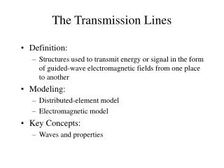
Preliminaries Generators and loads are connected together through transmission lines transporting electric power from one place to another. Transmission line must, therefore, take power from generators, transmit it to location where it will be used, and then distribute it to individual consumers. A ROT: the power capability of a transmission line is proportional to the square of the voltage on the line. Therefore, very high voltage levels are used to transmit power over long distances. Once the power reaches the area where it will be used, it is stepped down to a lower voltages in distribution substations, and then delivered to customers through distribution lines.
Preliminaries Distribution line with no ground wire. Dual 345 kV transmission line
Preliminaries There two types of transmission lines: overhead lines and buriedcables.
Preliminaries An overhead transmission line usually consists of three conductors or bundles of conductors containing the three phases of the power system. The conductors are usually aluminum cable steel reinforced (ACSR), which are steel core (for strength) and aluminum wires (having low resistance) wrapped around the core.
Preliminaries In overhead transmission lines, the conductors are suspended from a pole or a tower via insulators.
Preliminaries In addition to phase conductors, a transmission line usually includes one or two steel wires called ground (shield) wires. These wires are electrically connected to the tower and to the ground, and, therefore, are at ground potential. In large transmission lines, these wires are located above the phase conductors, shielding them from lightning.
Preliminaries Cable lines are designed to be placed underground or under water. The conductors are insulated from one another and surrounded by protective sheath. Cable lines are usually more expensive and harder to maintain. They also have capacitance problem – not suitable for long distance. Transmission lines are characterized by a series resistance, inductance, and shunt capacitance per unit length. These values determine the power-carrying capacity of the transmission line and the voltage drop across it at full load.
Resistance The DC resistance of a conductor is given by (9.9.1) Where l is the length of conductor; A – cross-sectional area, is the resistivity of the conductor. Therefore, the DC resistance per meter of the conductor is (9.9.1) The resistivity of a conductor is a fundamental property of the material that the conductor is made from. It varies with both type and temperature of the material. At the same temperature, the resistivity of aluminum is higher than the resistivity of copper.
Resistance The resistivity increases linearly with temperature over normal range of temperatures. If the resistivity at one temperature is known, the resistivity at another temperature can be found from (9.10.1) Where T1 and T1 are temperature 1 in oC and the resistivity at that temperature, T2 and T2 are temperature 2 in oC and the resistivity at that temperature, and M is the temperature constant.
Resistance We notice that silver and copper would be among the best conductors. However, aluminum, being much cheaper and lighter, is used to make most of the transmission line conductors. Conductors made out of aluminum should have bigger diameter than copper conductors to offset the higher resistivity of the material and, therefore, support the necessary currents. AC resistance of a conductor is always higher than its DC resistance due to the skin effect forcing more current flow near the outer surface of the conductor. The higher the frequency of current, the more noticeable skin effect would be. At frequencies of our interest (50-60 Hz), however, skin effect is not very strong. Wire manufacturers usually supply tables of resistance per unit length at common frequencies (50 and 60 Hz). Therefore, the resistance can be determined from such tables.
Inductance and inductive reactance The series inductance of a transmission line consists of two components: internal and external inductances, which are due the magnetic flux inside and outside the conductor respectively. The inductance of a transmission line is defined as the number of flux linkages [Wb-turns]produced per ampere of current flowing through the line: (9.12.1) 1. Internal inductance: Consider a conductor of radius r carrying a current I. At a distance x from the center of this conductor, the magnetic field intensity Hx can be found from Ampere’s law: (9.12.2)
Inductance and inductive reactance Where Hx is the magnetic field intensity at each point along a closed path, dl is a unit vector along that path and Ix is the net current enclosed in the path. For the homogeneous materials and a circular path of radius x, the magnitude of Hx is constant, and dl is always parallel to Hx. Therefore: (9.13.1) Assuming next that the current is distributed uniformly in the conductor: (9.13.2) Thus, the magnetic intensity at radius x inside the conductor is (9.13.3)
Inductance and inductive reactance The flux density at a distance x from the center of the conductor is (9.14.1) The differential magnetic flux contained in a circular tube of thickness dx and at a distance x from the center of the conductor is (9.14.2) The flux linkages per meter of length due to flux in the tube is the product of the differential flux and the fraction of current linked: (9.14.3)
Inductance and inductive reactance The total internal flux linkages per meter can be found via integration… (9.15.1) Therefore, the internal inductance per meter is (9.15.2) If the relative permeability of the conductor is 1 (non-ferromagnetic materials, such as copper and aluminum), the inductance per meter reduces to (9.15.3)
External inductance between 2 points outside of the line To find the inductance external to a conductor, we need to calculate the flux linkages of the conductor due only the portion of flux between two points P1 and P2 that lie at distances D1 and D2 from the center of the conductor. In the external to the conductor region, the magnetic intensity at a distance x from the center of conductor is (9.16.1) since all the current is within the tube. The flux density at a distance x from the center of conductor is (9.16.2)
External inductance between 2 points outside of the line The differential magnetic flux contained in a circular tube of thickness dx and at a distance x from the center of the conductor is (9.17.1) The flux links the full current carried by the conductor, therefore: (9.17.2) The total external flux linkages per meter can be found via integration… (9.17.3) The external inductance per meter is (9.17.4)
Inductance of a single-phase 2-wire transmission line We determine next the series inductance of a single-phase line consisting of two conductors of radii r spaced by a distance D and both carrying currents of magnitude I flowing into the page in the left-hand conductor and out of the page in the right-hand conductor. Considering two circular integration paths, we notice that the line integral along x1 produces a net magnetic intensity since a non-zero net current is enclosed by x1. Thus: (9.18.1) Since the path of radius x2 encloses both conductors and the currents are equal and opposite, the net current enclosed is 0 and, therefore, there are no contributions to the total inductance from the magnetic fields at distances greater than D.
Inductance of a single-phase 2-wire transmission line The total inductance of a wire per unit length in this transmission line is a sum of the internal inductance and the external inductance between the conductor surface (r) and the separation distance (D): (9.19.1) By symmetry, the total inductance of the other wire is the same, therefore, the total inductance of a two-wire transmission line is (9.19.2) Where r is the radius of each conductor and D is the distance between conductors.
Inductance of a transmission line Equations similar to (9.19.2) can be derived for three-phase lines and for lines with more phases… In most of the practical situations, the inductance of the transmission line can be found from tables supplied by line developers. • Analysis of (9.19.2) shows that: • The greater the spacing between the phases of a transmission line, the greater the inductance of the line. Since the phases of a high-voltage overhead transmission line must be spaced further apart to ensure proper insulation, a high-voltage line will have a higher inductance than a low-voltage line. Since the spacing between lines in buried cables is very small, series inductance of cables is much smaller than the inductance of overhead lines. • The greater the radius of the conductors in a transmission line, the lower the inductance of the line. In practical transmission lines, instead of using heavy and inflexible conductors of large radii, two and more conductors are bundled together to approximate a large diameter conductor. The more conductors included in the bundle, the better the approximation becomes. Bundles are often used in the high-voltage transmission lines.
Inductance of a transmission line A two-conductor bundle A four-conductor bundle
Inductive reactance of a line The series inductive reactance of a transmission line depends on both the inductance of the line and the frequency of the power system. Denoting the inductance per unit length as l, the inductive reactance per unit length will be (9.22.1) where f is the power system frequency. Therefore, the total series inductive reactance of a transmission line can be found as (9.22.2) where d is the length of the line.
Capacitance and capacitive reactance Since a voltage V is applied to a pair of conductors separated by a dielectric (air), charges of equal magnitude but opposite sign will accumulate on the conductors: (9.23.1) Where C is the capacitance between the pair of conductors. In AC power systems, a transmission line carries a time-varying voltage different in each phase. This time-varying voltage causes the changes in charges stored on conductors. Changing charges produce a changing current, which will increase the current through the transmission line and affect the power factor and voltage drop of the line. This changing current will flow in a transmission line even if it is open circuited.
Capacitance and capacitive reactance The capacitance of the transmission line can be found using the Gauss’s law: (9.24.1) where A specifies a closed surface; dA is the unit vector normal to the surface; q is the charge inside the surface; D is the electric flux density at the surface: (9.24.2) where E is the electric field intensity at that point; is the permittivity of the material: (9.24.3) Relative permittivity of the material The permittivity of free space 0 = 8.8510-12 F/m
Capacitance and capacitive reactance Electric flux lines radiate uniformly outwards from the surface of the conductor with a positive charge on its surface. In this case, the flux density vector D is always parallel to the normal vector dA and is constant at all points around a path of constant radius r. Therefore: (9.25.1) were l is the length of conductor; q is the charge density; Q is the total charge on the conductor. Then the flux density is (9.25.2) The electric field intensity is (9.25.3)
Capacitance and capacitive reactance The potential difference between two points P1 and P2 can be found as (9.26.1) where dl is a differential element tangential to the integration path between P1 and P2. The path is irrelevant. Selection of path can simplify calculations. For P1 - Pint, vectors E and dl are parallel; therefore, Edl = Edx. For Pint – P2 vectors are orthogonal, therefore Edl = 0. (9.26.2)
Capacitance of a single phase two-wire transmission line The potential difference due to the charge on conductor a can be found as (9.27.1) Similarly, the potential difference due to the charge on conductor b is (9.27.2) or (9.27.3)
Capacitance of a single phase two-wire transmission line The total voltage between the lines is (9.28.1) Since q1 = q2 = q, the equation reduces to (9.28.2) The capacitance per unit length between the two conductors of the line is (9.28.3)
Capacitance of a single phase two-wire transmission line Thus: (9.29.1) Which is the capacitance per unit length of a single-phase two-wire transmission line. The potential difference between each conductor and the ground (or neutral) is one half of the potential difference between the two conductors. Therefore, the capacitance to ground of this single-phase transmission line will be (9.29.2)
Capacitance of a single phase two-wire transmission line Similarly, the expressions for capacitance of three-phase lines (and for lines with more than 3 phases) can be derived. Similarly to the inductance, the capacitance of the transmission line can be found from tables supplied by line developers. • Analysis of (9.29.1) shows that: • The greater the spacing between the phases of a transmission line, the lower the capacitance of the line. Since the phases of a high-voltage overhead transmission line must be spaced further apart to ensure proper insulation, a high-voltage line will have a lower capacitance than a low-voltage line. Since the spacing between lines in buried cables is very small, shunt capacitance of cables is much larger than the capacitance of overhead lines. Cable lines are normally used for short transmission lines (to min capacitance) in urban areas. • The greater the radius of the conductors in a transmission line, the higher the capacitance of the line. Therefore, bundling increases the capacitance. Good transmission line is a compromise among the requirements for low series inductance, low shunt capacitance, and a large enough separation to provide insulation between the phases.
Shunt capacitive admittance The shunt capacitive admittance of a transmission line depends on both the capacitance of the line and the frequency of the power system. Denoting the capacitance per unit length as c, the shunt admittance per unit length will be (9.31.1) The total shunt capacitive admittance therefore is (9.31.2) where d is the length of the line. The corresponding capacitive reactance is the reciprocal to the admittance: (9.31.3)
Example • Example 9.1: An 8000 V, 60 Hz, single-phase, transmission line consists of two hard-drawn aluminum conductors with a radius of 2 cm spaced 1.2 m apart. If the transmission line is 30 km long and the temperature of the conductors is 200C, • What is the series resistance per kilometer of this line? • What is the series inductance per kilometer of this line? • What is the shunt capacitance per kilometer of this line? • What is the total series reactance of this line? • What is the total shunt admittance of this line? a. The series resistance of the transmission line is Ignoring the skin effect, the resistivity of the line at 200 will be 2.8310-8 -m and the resistance per kilometer of the line is
Example b. The series inductance per kilometer of the transmission line is c. The shunt capacitance per kilometer of the transmission line is d. The series impedance per kilometer of the transmission line is Then the total series impedance of the line is
Example e. The shunt admittance per kilometer of the transmission line is The total shunt admittance will be The corresponding shunt capacitive reactance is
Transmission line models Unlike the electric machines studied so far, transmission lines are characterized by their distributed parameters: distributed resistance, inductance, and capacitance. The distributed series and shunt elements of the transmission line make it harder to model. Such parameters may be approximated by many small discrete resistors, capacitors, and inductors. However, this approach is not very practical, since it would require to solve for voltages and currents at all nodes along the line. We could also solve the exact differential equations for a line but this is also not very practical for large power systems with many lines.
Transmission line models Fortunately, certain simplifications can be used… Overhead transmission lines shorter than 80 km (50 miles) can be modeled as a series resistance and inductance, since the shunt capacitance can be neglected over short distances. The inductive reactance at 60 Hz for – overhead lines – is typically much larger than the resistance of the line. For medium-length lines (80-240 km), shunt capacitance should be taken into account. However, it can be modeled by two capacitors of a half of the line capacitance each. Lines longer than 240 km (150 miles) are long transmission lines and are to be discussed later.
Transmission line models The total series resistance, series reactance, and shunt admittance of a transmission line can be calculated as (9.37.1) (9.37.2) (9.37.3) where r, x, and y are resistance, reactance, and shunt admittance per unit length and d is the length of the transmission line. The values of r, x, and y can be computed from the line geometry or found in the reference tables for the specific transmission line.
Short transmission line The per-phase equivalent circuit of a short line VS and VR are the sending and receiving end voltages; IS and IR are the sending and receiving end currents. Assumption of no line admittance leads to (9.38.1) We can relate voltages through the Kirchhoff’s voltage law (9.38.2) (9.38.3) which is very similar to the equation derived for a synchronous generator.
Short transmission line: phasor diagram AC voltages are usually expressed as phasors. Load with lagging power factor. Load with unity power factor. Load with leading power factor. For a given source voltage VS and magnitude of the line current, the received voltage is lower for lagging loads and higher for leading loads.
Transmission line characteristics In real overhead transmission lines, the line reactance XL is normally much larger than the line resistance R; therefore, the line resistance is often neglected. We consider next some important transmission line characteristics… 1. The effect of load changes Assuming that a single generator supplies a single load through a transmission line, we consider consequences of increasing load. Assuming that the generator is ideal, an increase of load will increase a real and (or) reactive power drawn from the generator and, therefore, the line current, while the voltage and the current will be unchanged. 1) If more load is added with the same lagging power factor, the magnitude of the line current increases but the current remains at the same angle with respect to VR as before.
Transmission line characteristics The voltage drop across the reactance increases but stays at the same angle. Assuming zero line resistance and remembering that the source voltage has a constant magnitude: (9.41.1) voltage drop across reactance jXLI will stretch between VR and VS. Therefore, when a lagging load increases, the received voltage decreases sharply. 2) An increase in a unity PF load, on the other hand, will slightly decrease the received voltage at the end of the transmission line.
Transmission line characteristics 3) Finally, an increase in a load with leading PF increases the received (terminal) voltage of the transmission line. In a summary: • If lagging (inductive) loads are added at the end of a line, the voltage at the end of the transmission line decreases significantly – large positive VR. • If unity-PF (resistive) loads are added at the end of a line, the voltage at the end of the transmission line decreases slightly – small positive VR. • If leading (capacitive) loads are added at the end of a line, the voltage at the end of the transmission line increases– negative VR. The voltage regulation of a transmission line is (9.42.1) where Vnl and Vfl are the no-load and full-load voltages at the line output.
Transmission line characteristics 2. Power flow in a transmission line The real power input to a 3-phase transmission line can be computed as (9.43.1) where VS is the magnitude of the source (input) line-to-neutral voltage and VLL,S is the magnitude of the source (input) line-to-line voltage. Note that Y-connection is assumed! Similarly, the real output power from the transmission line is (9.43.2) The reactive power input to a 3-phase transmission line can be computed as (9.43.3)
Transmission line characteristics And the reactive output power is (9.44.1) The apparent power input to a 3-phase transmission line can be computed as (9.44.2) And the apparent output power is (9.44.3)
Transmission line characteristics If the resistance R is ignored, the output power of the transmission line can be simplified… A simplified phasor diagram of a transmission line indicating that IS = IR = I. We further observe that the vertical segment bc can be expressed as either VS sin or XLIcos. Therefore: (9.45.1) Then the output power of the transmission line equals to its input power: (9.45.2) Therefore, the power supplied by a transmission line depends on the angle between the phasors representing the input and output voltages.
Transmission line characteristics The maximum power supplied by the transmission line occurs when = 900: (9.46.1) This maximum power is called the steady-state stability limit of the transmission line. The real transmission lines have non-zero resistance and, therefore, overheat long before this point. Full-load angles of 250 are more typical for real transmission lines. Few interesting observations can be made from the power expressions: • The maximum power handling capability of a transmission line is a function of the square of its voltage. For instance, if all other parameters are equal, a 220 kV line will have 4 times the power handling capability of a 110 kV transmission line. • Therefore, it is beneficial to increase the voltage… However, very high voltages produce very strong EM fields (interferences) and may produce a corona – glowing of ionized air that substantially increases losses.
Transmission line characteristics 2. The maximum power handling capability of a transmission line is inversely proportional to its series reactance, which may be a serious problem for long transmission lines. Some very long lines include series capacitors to reduce the total series reactance and thus increase the total power handling capability of the line. 3. In a normal operation of a power system, the magnitudes of voltages VS and VR do not change much, therefore, the angle basically controls the power flowing through the line. It is possible to control power flow by placing a phase-shifting transformer at one end of the line and varying voltage phase. 3. Transmission line efficiency The efficiency of the transmission line is (9.47.1)
Transmission line characteristics 4. Transmission line ratings One of the main limiting factors in transmission line operation is its resistive heating. Since this heating is a function of the square of the current flowing through the line and does not depend on its phase angle, transmission lines are typically rated at a nominal voltage and apparent power. 5. Transmission line limits Several practical constrains limit the maximum real and reactive power that a transmission line can supply. The most important constrains are: 1. The maximum steady-state current must be limited to prevent the overheating in the transmission line. The power lost in a line is approximated as (9.48.1) The greater the current flow, the greater the resistive heating losses.
Transmission line characteristics 2. The voltage drop in a practical line should be limited to approximately 5%. In other words, the ratio of the magnitude of the receiving end voltage to the magnitude of the sending end voltage should be (9.49.1) This limit prevents excessive voltage variations in a power system. 3. The angle in a transmission line should typically be 300 ensuring that the power flow in the transmission line is well below the static stability limit and, therefore, the power system can handle transients. Any of these limits can be more or less important in different circumstances. In short lines, where series reactance X is relatively small, the resistive heating usually limits the power that the line can supply. In longer lines operating at lagging power factors, the voltage drop across the line is usually the limiting factor. In longer lines operating at leading power factors, the maximum angle can be the limiting f actor.
2-port networks and ABCD models A transmission line can be represented by a 2-port network – a network that can be isolated from the outside world by two connections (ports) as shown. If the network is linear, an elementary circuits theorem (analogous to Thevenin’s theorem) establishes the relationship between the sending and receiving end voltages and currents as (9.50.1) Here constants A and D are dimensionless, a constant B has units of , and a constant C is measured in siemens. These constants are sometimes referred to as generalized circuit constants, or ABCD constants.