Download
1 / 10
130 likes | 280 Vues
Explore derivation, computation, symmetries, and spectral estimation of Discrete Fourier Transform. Learn about Time Domain Windowing and practical MATLAB code implementation.

E N D
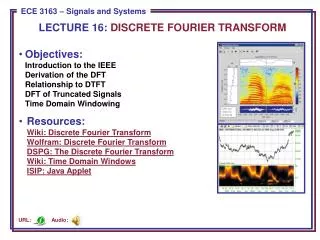
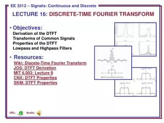
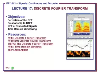
LECTURE 17: DISCRETE FOURIER TRANSFORM • Objectives:Derivation of the DFTRelationship to DTFTDFT of Truncated SignalsTime Domain Windowing • Resources:Wiki: Discrete Fourier TransformWolfram: Discrete Fourier TransformDSPG: The Discrete Fourier TransformWiki: Time Domain WindowsISIP: Java Applet URL:
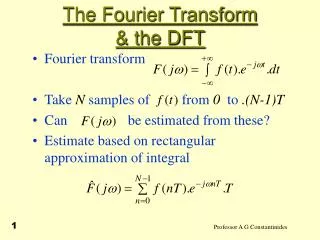
The Discrete-Time Fourier Transform • The Discrete-Time Fourier Transform: • Not practical for (real-time) computation on a digital computer. • Solution: limit the extent of the summation to N points and evaluate the continuous function of frequency at N equispaced points: • MATLAB code for the DFT: • The exponentials can be precomputedso that the DFT can be computedas a vector-matrix multiplication. • Later we will exploit the symmetryproperties of the exponential tospeed up the computation (e.g., fft()).
Computation of the DFT • Given the signal:
Symmetry • The magnitude and phase functions are even and odd respectively. • The DFT also has “circular” symmetry: • When N is even, |Xk| is symmetric about N/2. • The phase, Xk, has odd symmetry about N/2.
Inverse DFT • The inverse transform follows from the DT Fourier Series:
Relationship to the DTFT • q = 5 • The DFT and the DFT are related by: • If we define a pulse as: • The DFT is simply a sampling of theDTFT at equispaced points along thefrequency axis. • As N increases, the sampling becomesfiner. Note that this is true even whenq is constant increasing N is a way ofinterpolating the spectrum. • q=5, N = 22 • q = 5, N = 88
DFT of Truncated Signals • What if the signal is not time-limited?We can think of limiting the sum toN points as a truncation of the signal: • What are the implications of this in the frequency domain?(Hint: convolution) • Popular Windows: • Rectangular: • Generalized Hanning: • Triangular: • Rectangular • Generalized Hanning • Triangular
Impact on Spectral Estimation • The spectrum of a windowed sinewave is the convolution of two impulse functions with the frequency response of the window. • For two closely spaced sinewaves, there is “leakage” between each sinewave’s spectrum. • The impact of this leakage can be mitigated by using a window function with a narrower main lobe. • For example, consider the spectrum of three sinewaves computed using a rectangular and a Hamming window. • We see that for the same number of points, the spectrum produced by te Hamming window separates the sinewaves. • What is the computational cost?
Summary • Introduced the Discrete Fourier Transform as a truncated version of the Discrete-Time Fourier Transform. • Demonstrated both the forward and inverse transforms. • Explored the relationship to the DTFT. • Compared the spectrum of a pulse. • Discussed the effects of truncation on the spectrum. • Introduced the concept of time domain windowing and discussed the impact of windows in the frequency domain.