Download
1 / 51
510 likes | 804 Vues
Numerical Methods Discrete Fourier Transform Part: Discrete Fourier Transform http://numericalmethods.eng.usf.edu. For more details on this topic Go to http://numericalmethods.eng.usf.edu Click on Keyword Click on Discrete Fourier Transform . You are free.

E N D
Numerical MethodsDiscrete Fourier Transform Part: Discrete Fourier Transform http://numericalmethods.eng.usf.edu
For more details on this topic • Go to http://numericalmethods.eng.usf.edu • Click on Keyword • Click on Discrete Fourier Transform
You are free • to Share – to copy, distribute, display and perform the work • to Remix – to make derivative works
Under the following conditions • Attribution — You must attribute the work in the manner specified by the author or licensor (but not in any way that suggests that they endorse you or your use of the work). • Noncommercial — You may not use this work for commercial purposes. • Share Alike — If you alter, transform, or build upon this work, you may distribute the resulting work only under the same or similar license to this one.
Chapter 11.04 : Discrete Fourier Transform (DFT) Lecture # 8 Major: All Engineering Majors Authors: Duc Nguyen http://numericalmethods.eng.usf.edu Numerical Methods for STEM undergraduates 6/5/2014 http://numericalmethods.eng.usf.edu 5
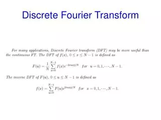
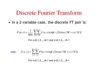
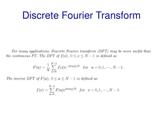
Discrete Fourier Transform Recalled the exponential form of Fourier series (see Eqs. 39, 41 in Ch. 11.02), one gets: (39, repeated) (41, repeated) 6 http://numericalmethods.eng.usf.edu
If time “ ” is discretized at Discrete Fourier Transform then Eq. (39) becomes: (1) http://numericalmethods.eng.usf.edu
the summation on “ ”, one Discrete Fourier Transform cont. To simplify the notation, define: (2) Then, Eq. (1) can be written as: (3) Multiplying both sides of Eq. (3) by , and performing obtains (note: l= integer number) 8 http://numericalmethods.eng.usf.edu
Discrete Fourier Transform cont. (4) (5) http://numericalmethods.eng.usf.edu
There are 2 possibilities for to be considered in Eq. (7) Discrete Fourier Transform cont. Switching the order of summations on the right-hand-side of Eq.(5), one obtains: (6) Define: (7) 10 http://numericalmethods.eng.usf.edu
Discrete Fourier Transform—Case 1 Case(1): is a multiple integer of N, such as: ; or where Thus, Eq. (7) becomes: (8) Hence: (9) 11 http://numericalmethods.eng.usf.edu
Case(2): is NOT a multiple integer of In this case, from Eq. (7) one has: Discrete Fourier Transform—Case 2 (10) Define: (11) 12 http://numericalmethods.eng.usf.edu
because is “NOT” a multiple integer of Discrete Fourier Transform—Case 2 Then, Eq. (10) can be expressed as: (12) http://numericalmethods.eng.usf.edu
if if Discrete Fourier Transform—Case 2 From mathematical handbooks, the right side of Eq. (12) represents the “geometric series”, and can be expressed as: (13) (14) 14 http://numericalmethods.eng.usf.edu
Because of Eq. (11), hence Eq. (14) should be used to compute . Thus: Discrete Fourier Transform—Case 2 (See Eq. (10)) (15) (16) http://numericalmethods.eng.usf.edu
Discrete Fourier Transform—Case 2 Substituting Eq. (16) into Eq. (15), one gets (17) Thus, combining the results of case 1 and case 2, we get (18) 16 http://numericalmethods.eng.usf.edu
The End http://numericalmethods.eng.usf.edu
Acknowledgement This instructional power point brought to you by Numerical Methods for STEM undergraduate http://numericalmethods.eng.usf.edu Committed to bringing numerical methods to the undergraduate
For instructional videos on other topics, go to http://numericalmethods.eng.usf.edu/videos/ This material is based upon work supported by the National Science Foundation under Grant # 0717624. Any opinions, findings, and conclusions or recommendations expressed in this material are those of the author(s) and do not necessarily reflect the views of the National Science Foundation.
Numerical MethodsDiscrete Fourier Transform Part: Discrete Fourier Transform http://numericalmethods.eng.usf.edu
For more details on this topic • Go to http://numericalmethods.eng.usf.edu • Click on Keyword • Click on Discrete Fourier Transform
You are free • to Share – to copy, distribute, display and perform the work • to Remix – to make derivative works
Under the following conditions • Attribution — You must attribute the work in the manner specified by the author or licensor (but not in any way that suggests that they endorse you or your use of the work). • Noncommercial — You may not use this work for commercial purposes. • Share Alike — If you alter, transform, or build upon this work, you may distribute the resulting work only under the same or similar license to this one.
Recall (where are integer numbers), And since must be in the range becomes Lecture # 9 Chapter 11.04: Discrete Fourier Transform (DFT) Substituting Eq.(18) into Eq.(7), and then referring to Eq.(6), one gets: (18A) Thus: http://numericalmethods.eng.usf.edu
and where Discrete Fourier Transform—Case 2 Eq. (18A) can, therefore, be simplified to (18B) Thus: (19) (1, repeated) 26 http://numericalmethods.eng.usf.edu
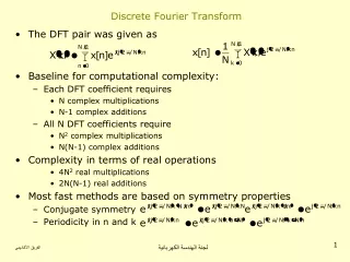
Discrete Fourier Transform cont. Equations (19) and (1) can be rewritten as (20) (21) 27 http://numericalmethods.eng.usf.edu
Discrete Fourier Transform cont. To avoid computation with “complex numbers”, Equation (20) can be expressed as (20A) where http://numericalmethods.eng.usf.edu
Discrete Fourier Transform cont. (20B) The above “complex number” equation is equivalent to the following 2 “real number” equations: (20C) (20D) 29 http://numericalmethods.eng.usf.edu
The End http://numericalmethods.eng.usf.edu
Acknowledgement This instructional power point brought to you by Numerical Methods for STEM undergraduate http://numericalmethods.eng.usf.edu Committed to bringing numerical methods to the undergraduate
For instructional videos on other topics, go to http://numericalmethods.eng.usf.edu/videos/ This material is based upon work supported by the National Science Foundation under Grant # 0717624. Any opinions, findings, and conclusions or recommendations expressed in this material are those of the author(s) and do not necessarily reflect the views of the National Science Foundation.
Numerical MethodsDiscrete Fourier Transform Part: Aliasing Phenomenon Nyquist Samples, Nyquist ratehttp://numericalmethods.eng.usf.edu
For more details on this topic • Go to http://numericalmethods.eng.usf.edu • Click on Keyword • Click on Discrete Fourier Transform
You are free • to Share – to copy, distribute, display and perform the work • to Remix – to make derivative works
Under the following conditions • Attribution — You must attribute the work in the manner specified by the author or licensor (but not in any way that suggests that they endorse you or your use of the work). • Noncommercial — You may not use this work for commercial purposes. • Share Alike — If you alter, transform, or build upon this work, you may distribute the resulting work only under the same or similar license to this one.
When a function which may represent the signals from some real-life phenomenon (shown in Figure 1), is sampled, it basically converts that function into a sequence at discrete locations of Lecture # 10 Chapter 11.04: Aliasing Phenomenon, Nyquist samples, Nyquist rate (Contd.) Figure 1: Function to be sampled and “Aliased” sample problem. 38 http://numericalmethods.eng.usf.edu
Thus, represents the value of where is the location of the first sample In Figure 1, the samples have been taken with a fairly large Thus, these sequence of discrete data will not be able to recover the original signal function Aliasing Phenomenon, Nyquist samples, Nyquist rate cont. 39 http://numericalmethods.eng.usf.edu
These piecewise linear interpolation (or other interpolation schemes) will NOT produce a curve which closely resembles the original function . This is the case where the data has been “ALIASED”. For example, if all discrete values of were connected by piecewise linear fashion, then a nearly horizontal straight line will occur between through and through respectively (See Figure 1). Aliasing Phenomenon, Nyquist samples, Nyquist rate cont. 40 http://numericalmethods.eng.usf.edu
Another potential difficulty in sampling the function is called “windowing” problem. As indicated in Figure 2, while is small enough so that a piecewise linear interpolation for connecting these discrete values will adequately resemble the original function , however, only a portion of the function has been sampled (from through ) rather than the entire one. In other words, one has placed a “window” over the function. “Windowing” phenomenon 41 http://numericalmethods.eng.usf.edu
Figure 2. Function to be sampled and “windowing” sample problem. “Windowing” phenomenon cont. 42 http://numericalmethods.eng.usf.edu
Figure 3. Frequency of sampling rate versus maximum frequency content In order to satisfy the frequency ( ) should be between points A and B of Figure 3. “Nyquist samples, Nyquist rate” 43 http://numericalmethods.eng.usf.edu
“Nyquist samples, Nyquist rate” Hence: which implies: Physically, the above equation states that one must have at least 2 samples per cycle of the highest frequency component present (Nyquist samples, Nyquist rate). 44 http://numericalmethods.eng.usf.edu
Figure 4. Correctly reconstructed signal. “Nyquist samples, Nyquist rate” 45 http://numericalmethods.eng.usf.edu
In Figure 4, a sinusoidal signal is sampled at the rate of 6 samples per 1 cycle (or ). Since this sampling rate does satisfy the sampling theorem requirement of , the reconstructed signal does correctly represent the original signal. “Nyquist samples, Nyquist rate” 46 http://numericalmethods.eng.usf.edu
In Figure 5 a sinusoidal signal is sampled at the rate of 6 samples per 4 cycles Since this sampling rate does NOT satisfy the requirement the reconstructed signal was wrongly represent the original signal! Figure 5. Wrongly reconstructed signal. “Nyquist samples, Nyquist rate” 47 http://numericalmethods.eng.usf.edu
The End http://numericalmethods.eng.usf.edu
Acknowledgement This instructional power point brought to you by Numerical Methods for STEM undergraduate http://numericalmethods.eng.usf.edu Committed to bringing numerical methods to the undergraduate
For instructional videos on other topics, go to http://numericalmethods.eng.usf.edu/videos/ This material is based upon work supported by the National Science Foundation under Grant # 0717624. Any opinions, findings, and conclusions or recommendations expressed in this material are those of the author(s) and do not necessarily reflect the views of the National Science Foundation.