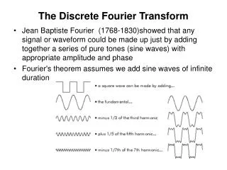
The Discrete Fourier Transform
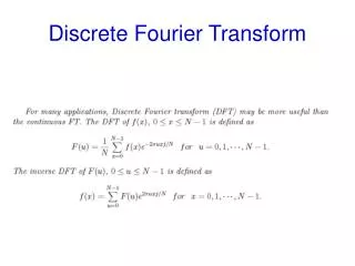
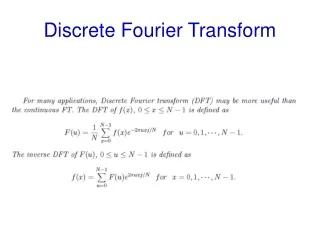
The Discrete Fourier Transform. The spectrum of a sampled function is given by. where – p < w < p or 0 < w < 2p . Since it impossible to carry-out the summation from n=- to , let us consider a truncated version of x[n]:. The corresponding Fourier transform is.


The Discrete Fourier Transform
E N D
Presentation Transcript
The spectrum of a sampled function is given by where –p < w < p or 0 < w < 2p.
Since it impossible to carry-out the summation from n=- to , let us consider a truncated version of x[n]: The corresponding Fourier transform is
Because the series is truncated, the resultant spectrum will exhibit Gibb’s phenomenon: there will be ripples near the edges of the spectrum.
Now let us choose Nfrequency points from w = 0 to 2p: When plugged into ejw, these values correspond to points along the unit circle.
As an example, if N = 4, we have The values of ejw are shown on the following slide.
Im Re
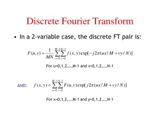
When we insert into we get
This function of k is the definition of the discrete Fourier transform.
Example: Find the discrete Fourier transform of x[n]=d[n], for N=4. Solution: we have only four time samples and four frequency samples. The values of the time samples are 1 0 0 0 (for n=0, 1, 2, 3). Inserting these values into the DFT definition, we have
Note that this result is independent of k. The result is consistent with the Fourier transform of a delta function.
Example: Find the discrete Fourier transform of x[n]=1, for N=4. Solution: as before, we have only four time samples and four frequency samples. The values of the time samples are 1 1 1 1 (for n=0, 1, 2, 3). Inserting these values into the DFT definition, we have
This result is dependent upon k. To perform the rest of the calculations, it is good to have our circle of value of e-j2pnk/4
Im Re
The previous example suggests that the discrete Fourier transform can be calculated using a matrix equation:
For the previous examples we have x[n]=d[n]
In both cases the results are consistent with Fourier transforms: the Fourier transform of an impulse is a constant (white) spectrum, and the Fourier transform of a constant is an impulse in frequency domain (just a D.C. component). Suppose that we found the DFT of x[n] = {1 –1 1 –1}.
We get the Fourier transform of a sinewave at half the sampling frequency: k=2 (for N = 4) corresponds to w=p, or W=Ws/2. In general we have
Example: Suppose we sample a 2 kHz sinewave at 8000 samples/second. If we perform a 1024-point DFT, where are the spikes in the transform? Solution: There will also be a spike at k=1024-256=768.
We can perform discrete Fourier transformations in MATLAB using the function fft(). In MATLAB, as in other software packages, the discrete Fourier transform is implemented using an algorithm called a fast Fourier transform. The previous examples were done using MATLAB as will be shown on the following slides.
x[n] = d[n] >> x = [1 0 0 0]; >> X = fft(x) X = 1 1 1 1
x[n] = 1 >> x = [1 1 1 1]; >> X = fft(x) X = 4 0 0 0
x[n] = {1 –1 1 –1} >> x = [1 -1 1 -1]; >> X = fft(x) X = 0 0 4 0
x is a 2 kHz sinewave >> n = 0:1023; >> t = n/8000; >> x = sin(2000*2*pi*t); >> X = fft(x); >> plot(n,abs(X));
Example: Suppose we sample a sinewave at 16000 samples/second. After performing a 2048-point DFT, we have frequency spikes at k=128 and k = 1920. Find the frequency of the sinewave. Solution:
Example: Suppose we sample the following signal at 4000 samples/sec: If we take a 512-point DFT, where are the frequency spikes? Solution: We find k for each of the two frequencies: f1 = 500, f2 = 250.
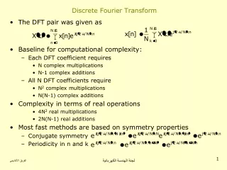
The Fast Fourier Transform An N-point DFT takes N2 complex multiplications and N2 complex additions. For large values of N, the number of computations becomes very large. A number of computationally-efficient algorithms have been developed called fast Fourier transforms, whose number of computations is far less than N2. The key to the efficiency is in the exploitation of the properties of e-j2pkn/N.
Now, suppose we rearrange the orderof the x[n] (time-domain) values:
This reordering lends itself to a repartitioning of the matrices:
Adopting further notation for the partitioned matrix, we have where The W11 matrix is a two-point DFT.
The W12 matrix is a two-point DFT with the second row (output) multiplied by W1. We denote this operation by The W21 matrix is the same as the W11 matrix—a two-point DFT.
and The W22 matrix is a two-point DFT with the first row multiplied by W2, and the second row (output) multiplied by W3:
Xfirst half N/2 + xeven [1, W1] Xsecond half N/2 + xodd [W2,W3]
Further detail can be given to the block diagram: N/2 X0 + xeven X1 + W1 N/2 X2 + xodd W2 X3 + W3
Finally, x0 X0 + + x2 X1 + + W2 W1 x1 X2 + + W2 x3 X3 + + W2 W3
The resultant algorithm is called a [decimation in time, radix-2] fast Fourier transform (FFT) and uses fewer complex multiplications than a conventional discrete Fourier transform (DFT). The [radix-2] FFT algorithm consists of a number of operations that look like this: + a + b This operation is called a butterflyand consists of two (complex) additions and two (complex) multiplications.
This general computational idea can be extended to higher-order DFT’s.
For example, an 8-point DFT can be constructed from two 4-point DFT’s and four butterflies to connect their outputs. A 16-point DFT can be constructed from two 8-point DFT’s and eight butterflies. The savings in number of computations can be seen in the following table.
The number of complex multiplications to perform an N-point DFT using the conventional (DFT) algorithm and the FFT algorithm.
Exercise: Construct an 8-point [decimation-in-time, radix-2] FFT from two 4-point FFT’s (already constructed). Verify that the number of (complex) multiplications is 24.
There are other types of fast Fourier transforms. The FFT just developed was created by reordering the time samples into even and odd parts. A second type of FFT reorders the frequency samples into even and odd parts. The first FFT algorithm is called a decimation-in-time FFT. The second algorithm is called a decimation-in-frequency FFT.