LECTURE 32: SECOND-ORDER SYSTEMS
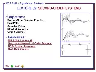
LECTURE 32: SECOND-ORDER SYSTEMS. Objectives: Second-Order Transfer Function Real Poles Complex Poles Effect of Damping Circuit Example Resources: MIT 6.003: Lecture 18 GW: Underdamped 2 nd -Order Systems CRB: System Response RVJ: RLC Circuits. Audio:. URL:. Second-Order Transfer Function.

LECTURE 32: SECOND-ORDER SYSTEMS
E N D
Presentation Transcript
LECTURE 32: SECOND-ORDER SYSTEMS • Objectives:Second-Order Transfer FunctionReal PolesComplex PolesEffect of DampingCircuit Example • Resources:MIT 6.003: Lecture 18GW: Underdamped 2nd-Order SystemsCRB: System ResponseRVJ: RLC Circuits Audio: URL:
Second-Order Transfer Function • Recall our expression for a simple, 2nd-order differential equation: • Write this in terms of two parameters, and n, related to the poles: • From the quadratic equation: • There are three types of interestingbehavior of this system: Impulse Response Step Response
Step Response For Two Real Poles • When > 1, both poles arereal and distinct: • When = 1, both poles arereal (s=n) and repeated: • There are two componentsto this response:
Step Response For Two Real Poles (Cont.) Both Real and Repeated Two Real Poles • is referred to as the damping ratio because it controls the time constant of the impulse response (and the time to reach steady state); • n is the natural frequency and controls the frequency of oscillation (which we will see next for the case of two complex poles). • > 1: The system is considered overdamped because it does not achieve oscillation and simply directly approaches its steady-state value. • = 1: The system is considered critically damped because it is on the verge of oscillation.
Step Response For Two Complex Poles • When 0 < < 1, we have two complex conjugate poles: • The transfer function can be rewritten as: • The step response, after some simplification, can be written as: • Hence, the response of this system eventually settles to a steady-state value of 1. However, the response can overshoot the steady-state value and will oscillate around it, eventually settling in to its final value.
Analysis of the Step Response For Two Complex Poles Impulse Response • > 1: the overdamped system experiences an exponential rise and decay. Its asymptotic behavior is a decaying exponential. • = 1: the critically damped system has a fast rise time, and converges to the steady-state value in an exponetial fashion. • 0 < > 1: the underdamped system oscillates about the steady-state behavior at a frequency of d. • Note that you cannot control the rise time and the oscillation behavior independently! • What can we conclude about the frequency response of this system? Step Response
Implications in the s-Plane • Several important observations: • The pole locations are: • Since the frequencyresponse is computedalong the j-axis, we can see that the pole islocated at ±d. • The bandwidth of thepole is proportional to the distance from the j-axis, and is given by n. • For a fixed n, the range 0 < < 1describes a circle. We will make use of this concept in the next chapter when we discuss control systems. • What happens if is negative?
RC Circuit • Example: Find the response to asinewave:. • Solution: • Again we see the solution is the superposition of a transient and steady-state response. • The steady-state response could have been found by simply evaluating the Fourier transform at 0 and applying the magnitude scaling and phase shift to the input signal. Why? • The Fourier transform is given by:
Summary • Analyzed the behavior of stable 2nd-order systems. • Characterized these systems in terms of three possible behaviors: overdamped, critically-damped, or overdamped. • Discussed the implications of this in the time and frequency domains. • Analyzed the response of an RC circuit to a sinewave. • Next: Frequency response and Bode plots.