Weak Gravitational Lensing and Shapelets
330 likes | 537 Vues
Weak Gravitational Lensing and Shapelets. Alexandre Refregier (CEA Saclay) Collaborators: Richard Massey (Cambridge) David Bacon (Edinburgh) Tzu-Ching Chang (Columbia) Jason Rhodes (Caltech) Richard Ellis (Caltech) Jean-Luc Starck (CEA Saclay) Sandrine Pires (CEA Saclay)

Weak Gravitational Lensing and Shapelets
E N D
Presentation Transcript
Weak Gravitational Lensing and Shapelets Alexandre Refregier (CEA Saclay) Collaborators: Richard Massey (Cambridge) David Bacon (Edinburgh) Tzu-Ching Chang (Columbia) Jason Rhodes (Caltech) Richard Ellis (Caltech) Jean-Luc Starck (CEA Saclay) Sandrine Pires (CEA Saclay) IPAM/UCLA – January 2004
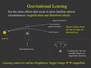
Distortion Matrix: Direct measure of the distribution of mass in the universe, as opposed to the distribution of light, as in other methods (eg. Galaxy surveys) Weak Gravitational Lensing Theory
Weak Lensing Shear Measurement unlensed background galaxies lensed background galaxies mass and shear distribution
Scientific Promise of Weak Lensing From the statistics of the shear field, weak lensing provides: • Mapping of the distribution of Dark Matter on various scales • Measurement of the evolution of structures • Measurement ofcosmological parameters, breaking degeneracies present in other methods (SNe, CMB) • Explore models beyond the standard osmological model (CDM) Jain, Seljak & White 1997, 25’x25’, SCDM
Cosmic Shear Surveys PSF anisotropy William Herschel Telescope La Palma, Canaries Deep Optical Images Bacon, Refregier & Ellis (2000) Correct for systematic effects: Bacon, Refregier, Clowe & Ellis (2001)
Shear Measurement Method KSB Method: (Kaiser, Squires & Broadhurst 1995) Quadrupole moments: Ellipticity: PSF Anisotropy correction: PSF Smear & Shear Calibration:
Cosmic Shear Measurements Shear variance in circular cells: 2()=<2> Bacon, Refregier & Ellis 2000* Bacon, Massey, Refregier, Ellis 2001 Kaiser et al. 2000* Maoli et al. 2000* Rhodes, Refregier & Groth 2001* Refregier, Rhodes & Groth 2002 van Waerbeke et al. 2000* van Waerbeke et al. 2001 Wittman et al. 2000* Hammerle et al. 2001* Hoekstra et al. 2002 * Brown et al. 2003 Hamana et al. 2003 * * not shown Jarvis et al. 2003 Casertano et al 2003* Rhodes et al 2004 +Rhodes et al.
Cosmological Constraints Hoekstra et al. 2002 E <Map2> B <Map2> (arcmin) E/B decomposition
Normalisation of the Power Spectrum Moderate disagreement among cosmic shear measurements (careful with marginalisation) Non-linear clustering corrections (Cf. Smith et al.) This could be due to residual systematics (shear normalisation? Cluster physics?) Agreement on average with cluster and CMB+LSS constraints Rhodes et al. 2003
The Shapelet Method > > | | > | = f00 + f01 +… < > | fnm = Refregier (2001) Refregier & Bacon (2001) also: Bernstein & Jarvis (2001) Decomposition of a galaxy image into shape components: Orthogonal Basis functions
Gauss-Hermite Basis Functions • Perturbations around a gaussian • Eigenfunctions of the Quantum Harmonic Oscillator • Coefficients are gaussian-weighted multipole moments • Capture a range of scales:
Polar Shapelets m=rotational oscillations (c.f. QM Lr momn) n=radial oscillations (c.f. QM energy) m=rotational oscillations (c.f. QM Lr momn) n=radial oscillations (c.f. QM energy)
HST galaxy Image Faithful description with a few shapelet coefficients
Image Compression Keep the top largest coefficients Achieve compression factors of 40-90 (for well resolved HST galaxies)
Fourier Transform and Convolution Convolution with a gaussian: Basis functions are invariant under Fourier transform (up to rescaling): Convolution: convolution tensor (analytic)
Coordinate Transformations • Transformations: • translations • rotations • shears • dilatations Eg: effect of shear on a galaxy image: simple operations in shapelet space
Difference Shear Measurement 1 = 0.1 2 = 0.1 ***To be replaced Shear Estimators: Combine estimators for minimum variance
Shear Measurement Shear recovery with ground based simulations: (Refregier & Bacon 2000) • Advantages: • All shape information used • Deconvolution recovers all available coefficients • Linear estimator noise biases are minimised • Minimum variance estimator Lensing signal is maximised • Analytic and mathematically well-defined • Stable and accurate
Simulating Space-Based Images • Decompose HDF galaxies into • shape components (“shapelets”) • Simulated galaxies are drawn from same • parameter space • Add noise, background, PSF, shear etc • as required a12 a11 • Ensures simulated images have same statistical properties as true HDF • Realistic illustration of SNAP science Massey, Refregier, Conselice & Bacon 2002
Shapelet Parameter Space -functions representing every HDF galaxy are placed into an n-dimensional parameter space, with each axis corresponding to a (polar) shapelet coefficient or size/magnitude. • The PDF is: • kernel-smoothed (assume a smooth underlying PDF exists) • Monte-Carlo sampled, to synthesise new ‘fake’ galaxies.
Smoothing in Shapelet Space smoothing param space smoothing param space Used in sims Real HDF Used in sims Real HDF Massey et al. (2002)
Test of the Simulations Blind test: run Sextractor and morphology software on HDFs and simulated images. Asymmetry Concentration
Weak Lensing Sensitivity Galaxies per arcmin2 RMS noise for the shear per galaxy RMS noise for the shear in 1 arcmin2 cell
Prospects for SNAP zS > 1.0 zS < 1.0 SNAP wide survey Rhodes et al. 2003, Massey et al. 2003, Refregier et al. 2003 SNAP will measure the evolution of the lensing power spectrum and set tight constraints on dark energy
input Dark Matter Mapping: Space observed Wavelets Wiener filter Starck, Refregier & Pires 2004
E: Lensing E/B Decomposition B: systematics
FIRST Radio Survey Faint Images of the Radio Sky at Twenty-cm • VLA B-array at 1.4 GHz • 10,000 deg2 area (~SDSS) • Resolution of 5”.4 • 90 Sources / deg at 1 mJy • < z > ~ 1 Becker,White Helfand (1995) White,Becker,Helfand,Gregg (1997) Snapshot survey Sparse UV sampling
Simulations Same observing condition as FIRST survey FWHMBeam Input Recovered Parallel code on COSMOS Origin2000: 23 Sources, ~ 200 parameters, ~18,000 visibilities ~1.5 GB memory, ~30 sec with 10 processors
Cosmological Constraints Chang, Refregier & Helfand 2004 Constraints consistent with current measurements of 8 and current knowledge of the redshifts of radio sources
Cosmic Shear with SKA • Square Kilometer Array: • an international project planned to be constructed in 2010 • FOV ~ 1 deg2 at 1.4 GHz, PSF ~ 0”.1 • Assuming 6 month’s observation: • 540 deg2 , beam FWH ~ 0”.1 • source number density: • ~100 sources arcmin-2 (~ HDF) • < z > =1 • se ~ 0.5
Conclusion • Weak Lensing provides a powerful measure of large-scale structure and cosmological parameters • Shapelets provides a high-precision shape measurement method required for future surveys • Other applicationsof shapelets: astrometry & photometry, study of galaxy morphology, de-projection, multi-color morphology • shapelet web page:http://www.ast.cam.ac.uk/~rjm/shapelets.html