Download
1 / 54
540 likes | 560 Vues
Explore the future of storage technology, from terabytes to yottabytes, and how it will shape our ability to store and analyze data. Discover the challenges and opportunities of managing and mining vast amounts of information.

E N D
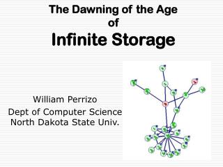
The Dawning of the AgeofInfinite Storage William Perrizo Dept of Computer Science North Dakota State Univ.
Google 10100 . . . Yotta 1024 Zetta 1021 Exa 1018 Peta 1015 Tera 1012 Giga 109 Mega 106 Kilo 103 • Tera Bytes are Here • 1 TB costs 1k$ to buy • 1 TB costs 300k$/y to own • Management & curation are expensive • Searching 1TB takes hours • I’m Terrified byTeraBytes • I’m Petrified by PetaBytes We are here • I’ll soon be Exafied byExaBytes • I’m too old to ever be Zettafied by ZettaBytes • But you may be in your lifetime • You may even be Yottafied by YottaBytes • You probably won’t ever be Googified byGoogiBytes • But one should “never say never”.
How much information is there? Yotta Zetta Exa Peta Tera Giga Mega Kilo Everything! Recorded • Soon everything can be recorded and indexed. • Most bytes will never be seen by humans. • Data summarization, trend detection, anomaly detection, data mining, are key technologies All Books MultiMedia All books (words) .Movie A Photo A Book 10-24 Yocto, 10-21 zepto, 10-18 atto, 10-15 femto, 10-12 pico, 10-9 nano, 10-6 micro, 10-3 milli
First Disk 1956 Me, at13. • IBM 305 RAMAC • 4 MB • 50x24” disks • 1200 rpm • 100 ms access • 35k$/y rent • Included computer & accounting software(tubes not transistors)
10 years later 30 MB 1.6 meters
12/1/1999 9/1/2000 9/1/2001 4/1/2002 11/4/2003 The Cost of Storage about 1K$/TB
E.g., A recent Purchase Order Company: NDSU Date: 8/7/03 System Board: Intel D865 GBFL system board w/LAN 800mhz FSB Processor: Intel Pentium 4 2.6 GHz Hard Drives: 4 x 250 GB IDE (total = 1 TB) Controller: Onboard IDE Controller 2nd IDE Controller: Video: Integrated Diskette Drive: 1.44 MB Memory: 4 GB 400 mhz memory CD/DVD Drive: DVD/CDRW Sound: Integrated AC97 Audio w/Soundmax Case: Performance Minitower ATX w/300 Watt PS Keyboard: Microsoft 104 Internet keyboard Mouse: Microsoft Intellimouse Optical Operating System: none Network Cards: Integrated Intel 10/100 Ethernet w/D845GEBV2L board Price:$2,899.00 Main expense is here
Kilo Mega Giga Tera Peta Exa Zetta Yotta Disk Evolution
MemexAs We May Think, Vannevar Bush, 1945 “A memex is a device in which an individual stores all his books, records, and communications, and which is mechanized so that it may be consulted with exceeding speed and flexibility” “yet if the user inserted 5000 pages of material a day it would take him hundreds of years to fill the repository, so that he can enter material freely”
The Personal TerabyteHow Will We Find Anything? • Need Queries, Indexing, Data Mining, Pivoting, Scalability, Backup, Replication, Online update, Set-oriented access. • If you don’t use a DBMS, you will implement one! • Need Data Mining, Machine Learning! • 80% of data is personal/individual • 20% is Corporate, Governmental SQL ++DBMS
Why Mining Data? • Parkinson’s Law (for data) Data expands to fill available storage (and then some) • Disk-storage version of Moore’s law Capacity 2 t / 9 months • Available storage doubles every 9 months!
Another More’s Law: More is Less The more volume, the less information. (AKA: Shannon’s Canon) A simple illustration: Which phone book is more helpful? BOOK-1BOOK-2 Name NumberName Number Smith 234-9816 Smith 234-9816 Jones 231-7237 Smith 231-7237 Jones 234-9816 Jones 231-7237
TIFF image Yield Map EOS Data Mining example This dataset is a 320 row and 320 column (102,400 pixels) spatial file with 5 feature attributes (B,G,R,NIR,Y). The (B,G,R,NIR) features are in the TIFF image and the Y (crop yield) feature is color coded in the Yield Map (blue=low; red=high) What is the relationship between the color intensities and yield? We can hypothsize: hi_greenandlow_red hi_yield which, while not a simply SQL query result, is not surprising. We could analyze the data to confirm this hypothesis, but: Data Mining is more than just confirming hypotheses The stronger rule, hi_NIR and low_red hi_yieldis not an SQL result and is surprising. Data Mining includes suggesting new hypotheses.
Another Precision Agriculture Example Grasshopper (or any pest) Infestation Prediction • Grasshopper caused significant economic loss each year. • Early infestation prediction is key to damage control. Association rule mining on remotely sensed imagery holds significant promise to achieve early detection. Can initial infestation be determined from RGB bands???
Gene1 Gene2, Gene3 Gene4, Gene 5, Gene6 Gene7, Gene8 Gene9 Clustering ARM Gene4 Gene7 Gene1 Gene3 Gene5 Gene2 Gene9 Gene6 Gene8 Gene Regulation Pathway Discovery • High confident rule mining on that cluster may discover the relationships among the genes in which the expression of one gene (e.g., Gene2) is regulated by others. Other genes (e.g., Gene4 and Gene7) may not be directly involved in regulating Gene2 and can therefore be excluded (more later). • Results of clustering may indicate, for instance, that nine genes are involved in a metabolic pathway.
Sensor Network Data Mining • Micro and Nano scale sensor blocks are being developed for sensing • Biological agents • Chemical agents • Motion detection • coatings deterioration • RF-tagging of inventory • Structural materials fatigue • There will be trillions++ of individual sensors creating mountains of data. • The data must be mined for it’s information.
Situation space ================================== \ CARRIER / Sensor Network Application: CubE for Active Situation Replication (CEASR) Nano-sensors dropped into the Situation space Drop or mortar “smart dust” sensors into the situation space to detect armour, chemical, biological, thermal…. Wherever a threshold level is senseda ping is sent for that location. .:.:.:.:..::….:. : …:…:: ..: . . :: :.:…: :..:..::. .:: ..:.::.. .:.:.:.:..::….:. : …:…:: ..: . . :: :.:…: :..:..::. .:: ..:.::.. .:.:.:.:..::….:. : …:…:: ..: . . :: :.:…: :..:..::. .:: ..:.::.. Using Alien Technology’s Fluidic Self-assembly (FSA) technology, clear plastic layers with embedded nano-LEDs at each voxel, are laminated into a viewing cube. The the pings are transmitted to the cube, using one Ptree, where the pattern is display on the cube. A more sophisticated CEASR device could sense and transmit intensity levels, lighting up the display voxel with the appropriate intensity. What data structure should be used? Standard horizontal record structures may be infeasible. We suggest one vertical P-tree. Soldier sees replica of sensed situation prior to entering space
Anthropology ApplicationDigital Archive Network for Anthropology (DANA)(data mine arthropological artifacts (shape, color, discovery location,…)
Data Mining? But also, some fool’s gold? Relevance and interestingness analysis, serves to assay those information and knowledge gems. Querying is asking specific questions and expecting specific answers. Data Miningis going into the MOUNTAIN of DATA, and returning with information gems.
visualization Pattern Evaluation and Assay Data Mining OLAP Classification Clustering ARM Loop backs Task-relevant Data Data Warehouse: cleaned, integrated, read-only, periodic, historical raw database Selection Feature extraction, tuple selection Data Cleaning/Integration: missing data, outliers, noise, errors Smart files Mountain of Raw Data Data Mining Process • Data mining: the core of the knowledge discovery process.
Fractals, … Standard querying Searching and Aggregating Data Prospecting Machine Learning Data Mining Association Rule Mining OLAP (rollup, drilldown, slice/dice.. Supervised Learning – classification regression SQL SELECT FROM WHERE Complex queries (nested, EXISTS..) FUZZY query, Search engines, BLAST searches Unsupervised Learning - clustering Walmart vs.KMart Data Mining versus Querying There is a whole spectrum of techniques to get information from data: On the Query end, much work is yet to be done(D. DeWitt, ACM SIGMOD Record’02). On the Data Mining end, the surface has barely beenscratched. But even those scratches had a great impact – One of the early scatchers became the biggest corporation in the world recently. A Non-scratcher filed for bankruptcy
Our Approach • Vertical, compressed data structures, variously called either Predicate-trees or Peano-trees (Ptrees in either case)1 processed horizontally • Ubiquitously, DBMSs process horizontal records vertically – thru SCANs • We propose processing vertical data structures (Ptree) horizontally - thru ANDs • Ptrees are data-mining-ready, compressed vertical data structures, which attempt to address the curses of scalability and curse of dimensionality. • How are Ptrees constructed? The next slides illustrates the construction of a set of BASIC P-TREES which represent a data file in a lossless, compressed datamining-ready way. 1 Ptree Technology is patent pending by North Dakota State University
A file, R(A1..An), contains horizontal structures (a set of horizontal records) Ptrees: vertically partition; then compress each vertical bit slice into a basic Ptree; R( A1 A2 A3 A4) R[A1] R[A2] R[A3] R[A4] 010 111 110 001 011 111 110 000 010 110 101 001 010 111 101 111 101 010 001 100 010 010 001 101 111 000 001 100 111 000 001 100 010 111 110 001 011 111 110 000 010 110 101 001 010 111 101 111 101 010 001 100 010 010 001 101 111 000 001 100 111 000 001 100 Horizontal structures (records) Scanned vertically R11 R12 R13 R21 R22 R23 R31 R32 R33 R41 R42 R43 0 1 0 1 1 1 1 1 0 0 0 1 0 1 1 1 1 1 1 1 0 0 0 0 0 1 0 1 1 0 1 0 1 0 0 1 0 1 0 1 1 1 1 0 1 1 1 1 1 0 1 0 1 0 0 0 1 1 0 0 0 1 0 0 1 0 0 0 1 1 0 1 1 1 1 0 0 0 0 0 1 1 0 0 1 1 1 0 0 0 0 0 1 1 0 0 0 1 0 1 0 0 0 0 1 0 01 0 1 0 0 1 01 1. Whole file is not pure1 0 2. 1st half is not pure1 0 0 0 0 0 1 01 P11 P12 P13 P21 P22 P23 P31 P32 P33 P41 P42 P43 3. 2nd half is not pure1 0 0 0 0 0 1 0 0 10 01 0 0 0 1 0 0 0 0 0 0 0 1 01 10 0 0 0 0 1 10 0 0 0 0 1 10 0 0 0 0 1 0 0 0 0 0 0 0 0 0 0 0 0 0 1 1 0 1 0 0 0 0 1 0 1 4. 1st half of 2nd half not 0 0 0 1 0 1 01 5. 2nd half of 2nd half is 1 0 1 0 6. 1st half of 1st of 2nd is 1 Eg, to count, 111 000 001 100s, use “pure111000001100”: 0 23-level P11^P12^P13^P’21^P’22^P’23^P’31^P’32^P33^P41^P’42^P’43 = 0 0 22-level=2 01 21-level 7. 2nd half of 1st of 2nd not 0 horizontally process these basic Ptrees using one multi-operand logical AND. processed vertically (vertical scans) R11 0 0 0 0 1 0 1 1 1-Dimensional Ptrees are built by recording the truth of the predicate “pure 1” recursively on halves, until there is purity, P11: But it is pure (pure0) so this branch ends
Can anyone build us a hardware ANDer for this Ptree AND? • A card for a Pentium-4 or Itanium (or Opteron or G5 or …) • An active network device (e.g., a modified ATM switch in which the inbuffer “load” code is modified to disable the clear-to-1’s – assuming buffer-load micro-code is clear-to-1’s followed by AND) • All optical device (ANDing on-the-fly with zero time delay???) • We envision a world-wide consortium of Beowulf clusters of such machines, so that the WWW can be data mined in parallel effectively??
Vertical Data Structures History • In the 1980’s vertical data structures were proposed for record-based workloads • Decomposition Storage Model (DSM, Copeland et al) • Attribute Transposed File (ATF) • Bit Transposed File (BTF, Wang et al); Viper • Band Sequential Format (BSQ) for Remotely Sensed Imagery • DSM and BTF initiatives have disappeared. Why? (next slide) • Vertical auxiliary and system structures • Domain & Request Vectors (DVA/ROLL/ROCC Perrizo, Shi, et al) • vertical system structures (query optimization & synchronization) • Bit Mapped Indexes (BMIs - very popular in Data Warehouses) • all indexes are vertical auxiliary structures really • BMI’s use bit maps (positional approach to IDing records) • other indexes use RID lists (keyword or value approach)
R( A1 A2 A3 A4) 010 111 110 001 011 111 110 000 010 110 101 001 010 111 101 111 101 010 001 100 010 010 001 101 111 000 001 100 111 000 001 100 R11 R12 R13 R21 R22 R23 R31 R32 R33 R41 R42 R43 R11 R12 R13 R21 R22 R23 R31 R32 R33 R41 R42 R43 0 1 0 1 1 1 1 1 0 0 0 1 0 1 1 1 1 1 1 1 0 0 0 0 0 1 0 1 1 0 1 0 1 0 0 1 0 1 0 1 1 1 1 0 1 1 1 1 1 0 1 0 1 0 0 0 1 1 0 0 0 1 0 0 1 0 0 0 1 1 0 1 1 1 1 0 0 0 0 0 1 1 0 0 1 1 1 0 0 0 0 0 1 1 0 0 0 1 0 1 1 1 1 1 0 0 0 1 0 1 1 1 1 1 1 1 0 0 0 0 0 1 0 1 1 0 1 0 1 0 0 1 0 1 0 1 1 1 1 0 1 1 1 1 1 0 1 0 1 0 0 0 1 1 0 0 0 1 0 0 1 0 0 0 1 1 0 1 1 1 1 0 0 0 0 0 1 1 0 0 1 1 1 0 0 0 0 0 1 1 0 0 1 Horizontal Processing of Vertical Structuresfor Record-based Workloads • For record-based workloads (e.g., SQL) (where the result is a set of records), changing the horizontal record structure and then having to reconstruct it, may introduce too much post processing? • For data mining workloads, the result is often a bit (Yes/No, True/False) or another unstructured result, where there is no reconstructive post processing?
Run Lists: Another way to handle vertical data. Generalized Ptrees using standard run length compression of vertical bit files (alternatively, using Lempl Zipf?, Golomb?, other?) R( A1 A2 A3 A4) -->R[A1] R[A2] R[A3] R[A4] 010 111 110 001 011 111 110 000 010 110 101 001 010 111 101 111 101 010 001 100 010 010 001 101 111 000 001 100 111 000 001 100 010 111 110 001 011 111 110 000 010 110 101 001 010 111 101 111 101 010 001 100 010 010 001 101 111 000 001 100 111 000 001 100 R11 0 0 0 0 1 0 1 1 • 1st run is Pure0 0:000 • truth:start R11 R12 R13 R21 R22 R23 R31 R32 R33 R41 R42 R43 0 1 0 1 1 1 1 1 0 0 0 1 0 1 1 1 1 1 1 1 0 0 0 0 0 1 0 1 1 0 1 0 1 0 0 1 0 1 0 1 1 1 1 0 1 1 1 1 1 0 1 0 1 0 0 0 1 1 0 0 0 1 0 0 1 0 0 0 1 1 0 1 1 1 1 0 0 0 0 0 1 1 0 0 1 1 1 0 0 0 0 0 1 1 0 0 2. 2nd run is Pure1 1:100 3.3rd run is Pure0 0:101 4. 4th run is Pure1 1:110 RL11 RL12 RL13 RL21 RL22 RL23 RL31 RL32 RL33 RL41 RL42 RL43 0:000 1:010 0:101 1:000 0:001 1:010 0:100 1:101 0:110 1:000 0:100 1:000 0:110 1:000 0:010 1:011 0:100 1:000 0:100 1:000 0:010 0:000 1:010 0:000 1:010 0:000 1:001 0:010 1:100 0:101 1:110 0:000 1:100 0:101 1:110 1:000 0:100 1:101 Eg, to count, 111 000 001 100s, use “pure111000001100”: RL11^RL12^RL13^RL’21^RL’22^RL’23^RL’31^RL’32^RL33^RL41^RL’42^RL’43 Run Lists: record the type and start-offset of pure runs. E.g., RL11: RL11 0:000 1:100 0:101 1:110 (to complement, flip purity bits)
YOUR DATA MINING YOUR DATA Data Integration Language DIL Ptree (Predicates) Query Language PQL DII (Data Integration Interface) DMI (Data Mining Interface) Data Repository lossless, compressed, distributed, vertically-structured P-tree database Architecture for the DataMIME™ System(DataMIMEtm = data mining, NO NOISE) (PDMS = P-tree Data Mining System) Internet
0 0 1 1 1 1 1 1 0 0 1 1 1 1 1 0 0 0 1 1 1 1 1 1 0 0 1 1 1 1 1 1 1 0 1 1 1 1 0 0 0 0 1 1 1 1 0 0 0 0 1 1 1 1 0 0 0 0 0 1 1 1 0 0 0 0 1 1 0 0 0 0 0 0 0 0 0 0 1 1 0 0 1 1 1 1 0 0 1 1 1 1 1 1 1 1 0 0 0 0 0 0 1 1 0 0 1 1 1 1 0 0 1 1 2-Dimensional Pure1-trees Node is 1 iff that quadrant is purely 1-bits, e.g., A bit-file(from, e.g., high-order bit of the RED band of a 2-D image) 1111110011111000111111001111111011110000111100001111000001110000 Which, in spatial raster order looks like: Run-length compress it into a quadrant tree using Peano order.
1=001 55 level-3 (pure=43) 0 1 1 1 1 1 1 0 0 1 1 1 1 1 0 0 0 1 1 1 1 1 1 0 0 1 1 1 1 1 1 1 0 1 1 1 1 1 1 1 1 1 1 1 1 1 1 1 1 1 1 1 1 1 1 1 1 0 1 1 1 1 1 1 1 0 1 2 3 1 16 0 0 15 0 1 16 level-2 2 3 0 0 0 4 1 0 1 0 4 0 4 3 0 1 4 level-1 3 7=111 1 1 1 1 1 1 0 0 0 0 0 0 1 1 0 0 1 1 1 1 0 0 1 level-0 1 2 . 2 . 3 ( 7, 1 ) 10.10.11 ( 111, 001 ) Count tree? Counts are what’s needed in DM, but P1-trees are more compressed and produce counts quickly. One can construct the Count-tree in which each inode counts 1s in that quadrant): • QID (Quadrant ID): e.g., 2.2.3 • Pure-1/Pure-0 quadrants • Root Count • Tree levels: 3, 2, 1, 0, with • Purity counts of 43 42 41 40 respectively • The Fan-out = 2dim = 4
Logical Operations on Ptrees(are used to get counts of any pattern) AND operation is faster than the bit-by-bit AND since, there are shortcuts (any pure0 operand node means result node is pure0.) (any pure1, copy subtree of the other operand to the result) e.g., only load quadrant 2 to AND Ptree1, Ptree2, etc. The more operands there are in the AND, the greater the benefit due to this shortcut (more pure0 nodes). Ptree 1 Ptree 2 AND result OR result
PM-tree1: m ______/ / \ \______ / / \ \ / / \ \ 1 m m 1 / / \ \ / / \ \ m 0 1 m 1 1 m 1 //|\ //|\ //|\ 1110 0010 1101 PM-tree2: m ______/ / \ \______ / / \ \ / / \ \ 1 0 m 0 / / \ \ 1 1 1 m //|\ 0100 AND Result: m ________ / / \ \___ / ____ / \ \ / / \ \ 1 0 m 0 / | \ \ 1 1 m m //|\ //|\ 1101 0100 Ptree: 55 ____________/ / \ \___________ / ___ / \___ \ / / \ \ 16 ____8__ _15__ 16 / / | \ / | \ \ 3 0 4 1 4 4 3 4 //|\ //|\ //|\ 1110 0010 1101 Complement: 9 ____________/ / \ \___________ / ___ / \___ \ / / \ \ 0 ____8__ __1__ 0 / / | \ / | \ \ 1 4 0 3 0 0 1 0 //|\ //|\ //|\ 0001 1101 0010 Ptree Algebra • And • Or • Complement • Other How to AND P-trees??? Depth-first Pure 1 path AND code 0 100 101 102 12 132 20 21 220 221 223 23 3 & 0 20 21 22 231 RESULT 0 0 0 20 20 20 21 21 21 220 221 223 22 220 221 223 23 231 231
Basic Ptrees (a Pure1-Trees predicate-tree for target bit of target attribute) e.g., P11, P12, …, P18, P21, …, P28, …, P71, …, P78 AND Target Attribute Target Bit Position Value Ptrees (predicate: quad is purely target value in target attribute) e.g., P1, 5 = P1, 101 = P11 AND P12’ AND P13 AND Target Attribute Target Value Tuple Ptrees (predicate: quad is purely target tuple) e.g., P(1, 2, 3) = P(001, 010, 111) = P1, 001 AND P2, 010 AND P3, 111 AND/OR Cube Ptrees (predicate: quad is purely in target cube (product of intervals) e.g., P([13],, [0.2]) = (P1,1 OR P1,2 OR P1,3) AND (P3,0 OR P3,1 OR P3,2) Basic, Value and Tuple Ptrees
Hilbert Ordering? • Hilbert ordering is 44-recursive tuning fork ordering (H-trees have fanout=16) • In 2-dimensions, Peano ordering is 22-recursive z-ordering (raster ordering)
down 0 1 2 3 4 5 6 7 8 9 A B C D E F 0 1 E F 3 2 C D 4 8 7 B 9 A 6 5 down . . . . . . 0 1 2 3 4 5 6 7 8 9 A B C D E F left up right down . . . . . . . . . . . . 0 1 2 3 4 5 6 7 8 9 A B C D E F 0 1 2 3 4 5 6 7 8 9 A B C D E F 0 1 2 3 4 5 6 7 8 9 A B C D E F 0 1 2 3 4 5 6 7 8 9 A B C D E F right down up 0 1 2 3 4 5 6 7 8 9 A B C D E F 0 1 2 3 4 5 6 7 8 9 A B C D E F 0 1 2 3 4 5 6 7 8 9 A B C D E F Coordinates of a tuning-fork (upper-left) depend on ancestry. (x,y) = (ggrrbb, ggrrbb). If your parent points Down and you are the H node in your tuning-fork, your 2-bit contribution is given by: row(x) col(y) 0 00 , 00 1 00 , 01 2 01 , 01 3 01 , 00 4 10 , 00 5 11 , 00 6 11 , 01 7 10 , 01 8 10 , 10 9 11 , 10 A 11 , 11 B 10 , 11 C 01 , 11 D 01 , 10 E 00 , 10 F 00 , 11 Lookup table for Up, Left, Right Parents are similar.
Ptree dimension • The dimension of the Ptree structure is a user chosen parameter • It can be chosen to fit the data dimension • Most datasets 1-D Ptrees (recursive halving) • 2-D Images 2-D Ptrees (recursive quartering) • 3-D Solids 3-D Ptrees (recursive eighth-ing) • Or dimension can be chosen based on other considerations • optimize compression • increase processing speed (next slide)
Unsorted relation Generalized Raster and Peano Sorting: generalizes to any table with numeric attributes (not just images). Raster Sorting: Attributes 1st Bit position 2nd Peano Sorting: Bit position 1st Attributes 2nd
Unsorted Generalized Raster Generalized Peano crop adult spam function mushroom Generalize Peano Sorting KNN speed improvement (using 5 UCI Machine Learning Repository data sets) 120 100 80 Time in Seconds 60 40 20 0
Astronomy Application:National Virtual Observatory data • What Ptree dimension and what ordering should be used for astronomical data? • Where all bodies are assumed to be on the surface of a sphere, the celestial sphere (shares equatorial plane with earth and has no specified radius) • Peano Triangle Mesh Tree (PTM-tree) • Peano Celestial Coordinate tree (PCCtree) • Uses (RA, dec) coordinates of the celestial sphere • RA=Recession Angle (longitudinal angle) • dec=declination (latitude angle)
Peano Triangular Mesh Tree (PTM-tree) • Similar to the Hierarchical Triangular Mesh (HTM) used in the Sloan Digital Sky Survey project. In both: • Sphere is divided into triangles • Triangle sides are always great circle segments. • PTM differs from HTM in the way in which they are ordered?
1,2 1,2 1,3,3 1,1,2 1,0 1,3,0 1,1,1 1,0 1,1,0 1,1 1,3 1,3,2 1,1 1.1.3 1,3,1 1,3 The difference between HTM and PTM-trees is in the ordering. 1 1 Ordering of PTM-tree Ordering of HTM Why use a different ordering?
dec RA PTM Triangulation of the Celestial Sphere Traverse southern hemisphere in the revere direction (just the identical pattern pushed down, arriving at the Southern neighbor of the start point – a globe-filling curve? This “Peano ordering” produces a sphere-surface filling curve with good continuity characteristics.
PTM triangulation – Next Level LRLR LRLR LRLR LRLR
PTM-triangulation - Next Level LRLR RLRL LRLR RLRL LRLR RLRL LRLR RLRL LRLR RLRL LRLR RLRL LRLR RLRL LRLR RLRL
Peano Celestial Coordinate Trees (PCCtrees) • Unlike PTM-trees which initially partition the sphere into the 8 faces of an octahedron: • the sphere is tranformed into a cylinder, • then into a rectangle, • then standard Peano ordering is used on the Celestial Coordinates. • Celestial Coordinates • RA is from 0 to 360o • dec is -90o to 90o.
PRAd e c 90o 0o -90o 0o 360o Z Z Z Z Z Z Z Z Z Z Z Z Z Z Z Z Z Z Z Z Z Z Z Z Z Z Z Z Z Z Z Z Z Z Z Z Z Z Z Z Z Z Z Z Z Z Z Z Z Z Z Z Z Z Z Z Z Z Z Z Z Z Z Z Z Z Z Z Z Z Z Z Z Z Z Z Z Z Z Z Z Z Z Z Z Z Z Z Z Z Z Z Z Z Z Z Z Z Z Z Z Z Z Z Z Z Z Z Z Z Z Z Z Z Z Z Z Z Z Z Z Z Z Z Z Z Z Z Z Z Z Z Z Z Z Z Z Z Z Z Z Z Z Z Z Z Z Z Z Z Z Z Z Z Z Z Z Z Z Z Z Z Z Z Z Z Z Z Z Z Z Z Z Z Z Z Z Z Z Z Z Z Z Z Z Z Z Z Z Z Z Z Z Z Z Z Z Z Z Z Z Z Z Z Z Z Z Z Z Z Z Z Z Z Z Z Z Z Z Z Z Z Z Z Z Z Z Z Z Z Z Z Z Z Z Z Z Z Z Z Z Z Z Z Z Z Z Z Z Z Z Z Z Z Z Z North Plane Z Z Z Z Z Z Z Z Z Z Z Z Z Z Z Z Z Z Z Z Z Z Z Z Z Z Z Z Z Z Z Z Z Z Z Z Z Z Z Z Z Z Z Z Z Z Z Z Z Z Z Z Z Z Z Z Z Z Z Z Z Z Z Z Z Z Z Z Z Z Z Z Z Z Z Z Z Z Z Z Z Z Z Z Z Z Z Z Z Z Z Z Z Z Z Z Z Z Z Z Z Z Z Z Z Z Z Z Z Z Z Z Z Z Z Z Z Z Z Z Z Z Z Z Z Z Z Z Z Z Z Z Z Z Z Z Z Z Z Z Z Z Z Z Z Z Z Z Z Z Z Z Z Z Z Z Z Z Z Z Z Z Z Z Z Z Z Z Z Z Z Z Z Z Z Z Z Z Z Z Z Z Z Z Z Z Z Z Z Z Z Z Z Z Z Z Z Z Z Z Z Z Z Z Z Z Z Z Z Z Z Z Z Z Z Z Z Z Z Z Z Z Z Z Z Z Z Z Z Z Z Z Z Z Z Z Z Z Z Z Z Z Z Z Z Z Z Z Z Z Z Z Z Z Z Z South Plane Plane Sphere Cylinder
SubCell-Location Myta Ribo Nucl Ribo 17, 78 12, 60 Mi, 40 1, 48 10, 75 0 0 7, 40 0 14, 65 0 0 16, 76 0 9, 45 Pl, 43 Function apop meio mito apop StopCodonDensity .1 .1 .1 .9 PolyA-Tail 1 1 0 0 Organism Species Vert Genome Size (million bp) Gene Dimension Table g0 g1 g2 g3 o0 human Homo sapiens 1 3000 Organism Dimension Table o1 fly Drosophila melanogaster 0 185 o2 1 1 1 1 1 0 0 1 0 1 0 0 1 0 1 1 o3 0 1 0 1 1 0 0 1 0 1 0 1 1 0 0 0 yeast Saccharomyces cerevisiae 0 12.1 e0 1 0 1 1 0 1 1 1 1 1 0 1 1 0 1 0 e0 mouse Mus musculus 1 3000 e1 e1 e2 e2 e3 LAB PI UNV STR CTY STZ ED AD S H M N e3 Experiment Dimension Table (MIAME) 3 2 a c h 1 2 2 b s h 0 2 4 a c a 1 2 4 a s a 1 PUBLIC (Ptree Unfied BioLogical InformtiCs Data Cube and Dimension Tables) Gene-OrganismDimension Table (chromosome,length) Gene-Experiment-Organism Cube (1 iff that gene from that organism expresses at a threshold level in that experiment.) many-to-many-to-many relationship
SubCell-Location Myta Ribo Nucl Ribo Function apop meio mito apop StopCodonDensity .1 .1 .1 .9 PolyA-Tail 1 1 0 0 Original Gene Dimension Table g0 g0 1 0 0 1 g1 0 1 1 g2 0 1 0 1 g3 1 0 g1 0 1 1 0 1 0 1 0 1 g2 1 0 0 0 1 0 0 g3 Myta Ribo Nuc l apop Me i o Mi to SCD 1 SCD 2 SCD 3 SCD 4 Poly-A G E N E 1 0 0 1 0 1 0 0 0 1 1 g0 0 1 0 0 1 0 0 0 0 1 1 g1 0 0 1 0 0 1 0 0 0 1 0 g2 0 1 0 1 0 0 1 0 0 1 0 g3 Boolean Gene Dimension Table (Binary) g3 g2 g1 g0 Protein-Protein Interaction Pyramid 0