Download
1 / 72
730 likes | 758 Vues
Explore the structure and scheduling of disks, disk management techniques, and the role of swap space and RAID. Learn about disk formatting, partitions, and various disk-scheduling algorithms for efficient disk I/O handling.

E N D
Outline • Disk Structure • Disk Scheduling • Disk Management • Swap-Space Management • RAID Structure • Disk Attachment • Stable-Storage Implementation • Tertiary Storage Devices
14.1 Disk Structure • Disk drives are addressed as large 1-dimensional arrays of logical blocks, where the logical block is the smallest unit of transfer. • The 1-dimensional array of logical blocks is mapped into the sectors of the disk sequentially. • Sector 0 is the first sector of the first track on the outermost cylinder. • Mapping proceeds (Cylinder, Track, Sector) • In practice, not always possible • Defective Sectors • # of tracks per cylinders is not a constant
Overview • OS is responsible for using hardware efficiently • For disk drives fast access time and disk bandwidth • Access time has two major components • Seek time is the time for the disk to move the heads to the cylinder containing the desired sector • Seek time seek distance • Minimize seek time • Rotational latency is the additional time waiting for the disk to rotate the desired sector to the disk head • Difficult for OS • Disk bandwidth is the total number of bytes transferred, divided by the total time between the first request for service and the completion of the last transfer
Overview (Cont.) • Several algorithms exist to schedule the servicing of disk I/O requests. • We illustrate them with a request queue (0-199). • 98, 183, 37, 122, 14, 124, 65, 67 • Head pointer 53
FCFS Illustration shows total head movement of 640 cylinders.
SSTF • Shortest-Seek-Time First (SSTF) • Selects the request with the minimum seek time from the current head position. • SSTF scheduling is a form of SJF scheduling; may cause starvation of some requests. • Remember that requests may arrive at any time • Illustration shows total head movement of 236 cylinders. • Not always optimal (how about 53371465…)
SCAN • The disk arm starts at one end of the disk, and moves toward the other end, servicing requests until it gets to the other end of the disk, where the head movement is reversed and servicing continues. • Sometimes called the elevator algorithm. • Illustration shows total head movement of 208 cylinders.
C-SCAN • Provides a more uniform wait time than SCAN. • The head moves from one end of the disk to the other, servicing requests as it goes. When it reaches the other end, however, it immediately returns to the beginning of the disk, without servicing any requests on the return trip. • Treats the cylinders as a circular list that wraps around from the last cylinder to the first one.
C-LOOK • Version of C-SCAN • Arm only goes as far as the last request in each direction, then reverses direction immediately, without first going all the way to the end of the disk.
Selecting a Disk-Scheduling Algorithm • SSTF is common and has a natural appeal • SCAN and C-SCAN perform better for systems that place a heavy load on the disk • Performance relies on the number and types of requests • Requests for disk service can be influenced by the file-allocation method (Contiguous? Linked? Indexed?) • The disk-scheduling algorithm should be written as a separate module of the operating system, allowing it to be replaced with a different algorithm if necessary • Either SSTF or LOOK is a reasonable choice for the default algorithm • Scheduled by OS? Scheduled by disk controller?
Disk Formatting • Low-level formatting, or physical formatting • Divide a disk into sectors that the controller can read and write • Special data structure for each sector: header – data – trailer • Header and Trailer contains information used by disk controller, such as a sector number and an Error-correcting code (ECC) • When the controller writes a sector of data, ECC is updated with a value calculated from all the bytes in the data area • When the sector is read, ECC is recalculated and is compared with the stored value verify the data is correct
Disk Partition • To use a disk to hold files, OS still needs to record its own data structures on the disk • Partition the disk into one or more groups of cylinders • Each partition can be treated as a separate disk • Logical formatting or “making a file system” • Store the initial file-system data structure onto the disk… • Maps of free and allocated space (FAT or inode) • Initial empty directory
Raw Disk • Use a disk partition as a large sequential array of logical blocks, with any file-system data structures • Raw I/O • Example • Database systems prefer raw I/O because it enables them to control the exact disk location where each database record is stored • Raw I/O bypasses all the file-system services, such as the buffer cache, file locking, pre-fetching, space allocation, file names, and directories
Boot Block • Boot block initializes system • Initialize CPU registers, device controllers, main memory • Start OS • A tiny bootstrap loader is stored in boot ROM • Bring a full bootstrap program from disk • Full bootstrap program is stored in boot blocks (fixed location) • The boot ROM instructs the disk controller to read the boot blocks into memory, and then start executing the code to load the entire OS
Bad Blocks • IDE • MS-DOS format : write a special value into the corresponding FAT entry for bad blocks • MS-DOS chkdsk : search and lock bad blocks
Bad Blocks – SCSI (Cont.) • Controller maintains a list of bad blocks on the disk • Low-level formatting spare sectors (OS don’t know) • Controller replaces each bad sector logically with one of the spare sectors(sector sparing, or forwarding) • Invalidate optimization by OS’s disk scheduling • Each cylinder has a few spare sectors
Bad Blocks – SCSI (Cont.) • Typical bad-sector transaction • OS tries to read logical block 87 • Controller calculates ECC and finds that it is bad. Report to OS • Reboot next time, a special command is run to tell the controller to replace the bad sector with a spare. • Whenever the system requests block 87, it is translated into the replacement sector’s address by the controller • Sector slipping: • Ex. 17 defective, spare follows sector 202 • Spare 202 201 … 18 17
Swap-Space Use • Swap-space — Virtual memory uses disk space as an extension of main memory • Main goal for the design and implementation of swap space is to provide the best throughput for VM system • Swap-space use • Swapping – use swap space to hold entire process image • Paging – simple store pages that have been pushed out of memory • Some OS may support multiple swap-space • Put on separate disks to balance the load • Better to overestimate than underestimate • If out of swap-space, some processes must be aborted or system crashed
Swap-Space Location • Swap-space: In a separate disk partition or in a normal file system (in UNIX, mkfile and swapadd (or fstab, vfstab)) • Convenience of allocation and management in the file system, and the performance of swapping in raw partitions • Swap-space in a file-system – simply a large file • Navigating the directory structure and the disk-allocation data structure takes time and potentially extra disk accesses • External fragmentation can greatly increase swapping times by forcing multiple seeks during reading or writing of a process image • Improve by caching in main memory and contiguous allocation • The cost of traversing FS data structure still remains
Swap-Space Location (Cont.) • Swap-space in a separate partition • Create a fixed amount of swap space during disk partitioning • Raw partition • A separate swap-space storage manager is used to allocate and de-allocate blocks • Use algorithms optimized for speed, rather than storage efficiency • Internal fragment may increase • Some OS supports both
Swap-space Management (Example) • 4.3BSD allocates swap space when process starts; holds text segment (the program) and data segment. • Kernel uses swap maps to track swap-space use • Solaris 1: text-segment pages (clean pages) are brought in from the file system and are thrown away if selected for paged out (more efficient) • Solaris 2: allocates swap space only when a page is forced out of physical memory, not when the virtual memory page is first created.
4.3 BSD Segment Swap Map Text-segment swap map 512K 512K 512K 71K Data-segment swap map 16K 32K 64K 128K
3 Important Aspects of Mass Storages • Reliability – is anything broken? • Redundancy is main hack to increased reliability • Availability – is the system still available to the user? • When single point of failure occurs is the rest of the system still usable? • ECC and various correction schemes help (but cannot improve reliability) • Data Integrity • You must know exactly what is lost when something goes wrong
Disk Arrays • Multiple arms improve throughput, but not necessarily improve latency • Striping • Spreading data over multiple disks • Reliability • General metric is N devices have 1/N reliability • Rule of thumb: MTTF of a disk is about 5 years • Hence need to add redundant disks to compensate • MTTR ::= mean time to repair (or replace) (hours for disks) • If MTTR is small then the array’s MTTF can be pushed out significantly with a fairly small redundancy factor
Disk Striping & Parity RAID Disk Striping Block Interleaved Parity RAID Data Block Data Block Parity :Subblock :Subblock
Data Striping • Bit-level striping: split the bit of each bytes across multiple disks • No. of disks can be a multiple of 8 or divides 8 • Block-level striping: blocks of a file are striped across multiple disks; with n disks, block i goes to disk (i mod n)+1 • Every disk participates in every access • Number of I/O per second is the same as a single disk • Number of data per second is improved • Provide high data-transfer rates, but not improve reliability
Redundant Arrays of Disks • Files are "striped" across multiple disks • Availability is improved by adding redundant disks • If a single disk fails, the lost information can be reconstructed from redundant information • Capacity penalty to store redundant information • Bandwidth penalty to update • RAID • Redundant Arrays of Inexpensive Disks • Redundant Arrays of Independent Disks • Hot Spare and Hot Swap
Raid Levels, Reliability, Overhead Redundantinformation
RAID Levels 0 - 1 • RAID 0 – No redundancy (Just block striping) • Cheap but unable to withstand even a single failure • RAID 1 – Mirroring • Each disk is fully duplicated onto its "shadow“ • Files written to both, if one fails flag it and get data from the mirror • Reads may be optimized – use the disk delivering the data first • Bandwidth sacrifice on write: Logical write = two physical writes • Most expensive solution: 100% capacity overhead • Targeted for high I/O rate , high availability environments • RAID 0+1 – stripe first, then mirror the stripe • RAID 1+0 – mirror first, then stripe the mirror
RAID Levels 2 & 3 • RAID 2 – Memory style ECC • Cuts down number of additional disks • Actual number of redundant disks will depend on correction model • RAID 2 is not used in practice • RAID 3 – Bit-interleaved parity • Reduce the cost of higher availability to 1/N (N = # of disks) • Use one additional redundant disk to hold parity information • Bit interleaving allows corrupted data to be reconstructed • Interesting trade off between increased time to recover from a failure and cost reduction due to decreased redundancy • Parity = sum of all relative disk blocks (module 2) • Hence all disks must be accessed on a write – potential bottleneck • Targeted for high bandwidth applications: Scientific, Image Processing
RAID Level 3: Parity Disk (Cont.) 10010011 11001101 10010011 . . . P logical record 1 0 0 1 0 0 1 1 1 1 0 0 1 1 0 1 1 0 0 1 0 0 1 1 1 1 0 0 1 1 1 1 Striped physical records 25% capacity cost for parity in this configuration (1/N)
RAID Levels 4 & 5 & 6 • RAID 4 – Block interleaved parity • Similar idea as RAID 3 but sum is on a per block basis • Hence only the parity disk and the target disk need be accessed • Problem still with concurrent writes since parity disk bottlenecks • RAID 5 – Block interleaved distributed parity • Parity blocks are interleaved and distributed on all disks • Hence parity blocks no longer reside on same disk • Probability of write collisions to a single drive are reduced • Hence higher performance in the consecutive write situation • RAID 6 • Similar to RAID 5, but stores extra redundant information to guard against multiple disk failures
Raid 4 & 5 Illustration RAID 4 RAID 5 Targeted for mixed applications A logical write becomes four physical I/Os
Disk Attachment • Disks may be attached one of two ways: • Host attached via an I/O port • Network attached via a network connection • Network-attached storage – implemented as a RAID array with software that implements RPC interface for NFS (UNIX machines) or CIFS (Windows machines) • Storage-area network – a private network (using storage protocols rather than network protocols) among servers and storage units, separate from LAN or WAN connecting clients and servers