Mass-Storage Structure
Mass-Storage Structure. Operating System Concepts chapter 12. CS 355 Operating Systems Dr. Matthew Wright. Background: Magnetic Disks. Rotate 60 to 200 times per second Transfer rate : rate at which data flows between drive and computer

Mass-Storage Structure
E N D
Presentation Transcript
Mass-Storage Structure Operating System Concepts chapter 12 CS 355 Operating Systems Dr. Matthew Wright
Background: Magnetic Disks • Rotate 60 to 200 times per second • Transfer rate: rate at which data flows between drive and computer • Positioning time (random-access time): time to move disk arm to desired cylinder (seek time) and time for desired sector to rotate under the disk head (rotational latency)
Disk Address Structure • Disks are addressed as a large 1-dimensional array of logical blocks (usually 512 bytes per logical block). • This array is mapped onto the sectors of the disk, usually with sector 0 on the outermost cylinder, then through that track, then through that cylinder, and then through the other cylinders working toward the center of the disk. • Converting logical addresses to cylinder and track numbers is difficult because: • Most disks have some defective sectors, which are replaced by spare sectors elsewhere on the disk. • The number of sectors per track might not be constant. • Constant linear velocity (CLV): tracks farther from center hold more bits, so disk rotates faster when reading these tracks to keep data rate constant (CSs, DVDs commonly use this method) • Constant angular velocity (CAV): rotational speed is constant, so bit density decreases from inner tracks to outer tracks to keep data rate constant
Disk Scheduling: FCFS • Simple, but generally doesn’t provide the fastest service • Example: suppose the read/write heads start on cylinder 53, and disk queue has requests for I/O to blocks on the following cylinders: • 98, 183, 37, 122, 14, 124, 65, 67 Diagram shows read/write head movement to service the requests FCFS. Total head movement spans 640 cylinders.
Disk Scheduling: SSTF • Shortest Seek Time First (SSTF): service the requests closest to the current position of the read/write heads • This is similar to SJF scheduling, and could starve some requests. • Example: heads at cylinder 53; disk request queue contains: • 98, 183, 37, 122, 14, 124, 65, 67 Diagram shows read/write head movement to service the requests SSTF. Total head movement spans 236 cylinders.
Disk Scheduling: SCAN • SCAN algorithm: disk heads start at one end, move towards the other end, then return, servicing requests along each way • Example: heads at cylinder 53 moving toward 0; request queue: • 98, 183, 37, 122, 14, 124, 65, 67 Diagram shows read/write head movement to service the requests with SCAN algorithm. Total head movement spans 236 cylinders.
Disk Scheduling: C-SCAN • Circular SCAN (C-SCAN): Disk heads start at one end, move towards the other end, servicing requests along each way. Disk heads return immediately to the first end without servicing requests, then repeat. • Example: heads at cylinder 53; request queue: • 98, 183, 37, 122, 14, 124, 65, 67 Diagram shows read/write head movement to service the requests with C-SCAN algorithm. Total head movement spans 383 cylinders.
Disk Scheduling: LOOK and C-LOOK • Like SPAN or C-SPAN algorithms, but only going as far as the last request in either direction. • Example: heads at cylinder 53; request queue: • 98, 183, 37, 122, 14, 124, 65, 67 Diagram shows read/write head movement to service the requests with C-SCAN algorithm. Total head movement spans 322 cylinders.
Selecting a Disk-Scheduling Algorithm • Which algorithm to choose? • SSTF is common and better than FCFS. • SCAN and C-SCAN perform better for systems that place a heavy load on the disk. • Performance depends on the number and types of requests, and the file-allocation method. • In general, either SSTF or LOOK is a reasonable choice for the default algorithm. • The disk-scheduling algorithm should be written as a separate module of the operating system, allowing it to be replaced with a different algorithm if necessary. • Why not let the controller built into the disk hardware manage the scheduling? • The disk hardware can take into account both seek time and rotational latency. • The OS may choose to mandate the disk scheduling to guarantee priority of certain types of I/O.
Disk Management • The Operating System may also be responsible for tasks such as disk formatting, booting from disk, and bad-block recovery. • Low-level formatting divides a disk into sectors, and is usually performed when the disk is manufactured. • Logical formatting creates a file system on the disk, and is done by the OS. • The OS maintains the boot blocks (or boot partition) that contain the bootstrap loader. • Bad blocks: disk blocks may fail • An error-correcting code (ECC) stored with each block can detect and possibly correct an error (if so, it is called a soft error). • Disks contain spare sectors which are substituted for bad sectors. • If the system cannot recover from the error, it is called a hard error, and manual intervention may be required.
Swap-Space Management • Recall that memory uses disk space as an extension of main memory; this disk space is called the swap space, even for systems that implement paging rather than pure swapping. • Swap-space can be: • A file in the normal file system: easy to implement, but slow in practice • A separate (raw) disk partition: requires a swap-space manager, but can be optimized for speed rather than storage efficiency • Linux allows the administrator to choose whether the swap space is in a file or in a raw disk partition.
RAID Structure • RAID: Redundant Array of Independent Disks or Redundant Array of Inexpensive Disks • In systems with large numbers of disks, disk failures are common. • Redundancy allows the recovery of data when disk(s) fail. • Mirroring: A logical disk consists of two physical disks, and every write is carried out on both disks. • Bit-level striping: Splits the bits of each byte across multiple disks, which improves the transfer rate. • Block-level striping: Splits blocks of a file across multiple disks, which improves the access rate for large files and allows for concurrent reads of small files. • A nonvolatile RAM (NVRAM) cache can be used to protect data waiting to be written in case a power failure occurs. • Are disk failures really independent? • What if multiple disks fail simultaneously?
RAID Levels • RAID level 0: non-redundant striping • Data striped at the block level, with no redundancy. • RAID level 1: mirrored disks • Two copies of data stored on different disks. • Data not striped. • Easy to recover data from one disk that fails • RAID 0 + 1: combines RAID levels 0 and 1 • Provides both • performance and • reliability.
RAID Levels • RAID level 2: error-correcting codes • Data striped across disks at the bit level. • Disks labeled P store extra bits that can be used to reconstruct data if one disk fails. • Requires fewer disks than RAID level 1. • Requires computation of the error-correction bits at every write, and failure recovery requires lots of reads and computation.
RAID Levels • RAID level 3: bit-interleaved parity • Data striped across disks at the bit level. • Since disk controllers can detect whether a sector has read correctly, a single parity bit can be used for error detection and correction. • As good as RAID level 2 in practice, but less expensive. • Still requires extra computation for parity bits. • RAID level 4: block-interleaved parity • Data striped across disks at the block level. • Stores parity blocks on a separate disk, which can be used to reconstruct the blocks on a single failed disk.
RAID Levels • RAID level 5: block-interleaved distributed parity • Data striped across disks at the • block level. • Spreads data and parity blocks across all disks. • Avoids possible overuse of a single parity disk, which could happen with RAID level 4. • RAID level 6: P + Q redundancy scheme • Like RAID level 5, but stores extra • redundant information to guard • against simultaneous failures of • multiple disks. • Uses error-correcting codes such as Reed-Solomon codes.
RAID Implementation • RAID can be implemented at various levels: • At the kernel of system software level • By the host bus-adapter hardware • By storage array hardware • In the Storage Area Network (SAN) by disk virtualization devices • Some RAID implementations include a hot spare: an extra disk that is not used until one disk fails, at which time the system automatically restores data onto the spare disk.
Stable-Storage Implementation • Stable storage: storage that never loses stored information. • Write-ahead logging (used to implement atomic transactions) requires stable storage. • To implement stable storage: • Replicate information on more than one nonvolatile storage media with independent failure modes. • Update information in a controlled manner to ensure that failure during an update will not leave all copies in a damaged state, and so that we can safely recover from a failure. • Three possible outcomes of a disk write: • Successful completion: all of the data written successfully • Partial failure: only some of the data written successfully • Total failure: occurs before write starts; previous data remains intact
Stable-Storage Implementation • Strategy: maintain two (identical) physical blocks for each logical block, on different disks, with error-detection bits for each block • A write operation proceeds as: • Write the information to the first physical block. • When the first write completes, then write the same information to the second physical block. • When the second write completes, then declare the operation successful. • During failure recovery, examine each pair of physical blocks: • If both are the same and neither contains a detectable error, then do nothing. • If one block contains a detectable error, then replace its contents with the other block. • If neither block contains a detectable error, but the values differ, then replace the contents of the first block with that of the second. • As long as both copies don’t fail simultaneously, we guarantee that a write operation will either succeed completely or result in no change.
Tertiary Storage • Most OSs handle removable disks almost exactly like fixed disks — a new cartridge is formatted and an empty file system is generated on the disk. • Tapes are presented as a raw storage medium, i.e., and application does not open a file on the tape, it opens the whole tape drive as a raw device. • Usually the tape drive is reserved for the exclusive use of that application. • Since the OS does not provide file system services, the application must decide how to use the array of blocks. • Since every application makes up its own rules for how to organize a tape, a tape full of data can generally only be used by the program that created it. • The issue of naming files on removable media is especially difficult when we want to write data on a removable cartridge on one computer, and then use the cartridge in another computer. • Contemporary OSs generally leave the name space problem unsolved for removable media, and depend on applications and users to figure out how to access and interpret the data. • Some kinds of removable media (e.g., CDs) are so well standardized that all computers use them the same way.