Algorithmic Verification of Concurrent Programs
Algorithmic Verification of Concurrent Programs. Shaz Qadeer Microsoft Research. Reliable concurrent software?. Correctness problem does program behave correctly for all inputs and all interleavings ? Bugs due to concurrency are insidious non-deterministic, timing dependent


Algorithmic Verification of Concurrent Programs
E N D
Presentation Transcript
Algorithmic Verification of Concurrent Programs Shaz Qadeer Microsoft Research
Reliable concurrent software? • Correctness problem • does program behave correctly for allinputs and allinterleavings? • Bugs due to concurrency are insidious • non-deterministic, timing dependent • data corruption, crashes • difficult to detect, reproduce, eliminate
Demo • Debugging concurrent programs is hard
Program verification • Program verification is undecidable • even for sequential programs • Concurrency does not make the worst-case complexity any worse • Why is verification of concurrent programs considered more difficult?
Undecidable problem! P satisfies S
Assertions: Provide contracts to decompose problem • into a collection of decidable problems • pre-condition and post-condition for each procedure • loop invariant for each loop P satisfies S • Abstractions: Provide an abstraction of the program • for which verification is decidable • Finite-state systems • finite automata • Infinite-state systems • pushdown automata, counter automata, timed automata, Petri nets
Assertions: an example ensures \result >= 0 ==> a[\result] == n ensures \result < 0 ==> forall j:int :: 0 <= j && j < a.length ==> a[j] != n int find(int a[ ], int n) { inti = 0; while (i < a.length) { if (a[i] == n) return i; i++; } return -1; }
Assertions: an example ensures \result >= 0 ==> a[\result] == n ensures \result < 0 ==> forall j:int :: 0 <= j && j < a.length ==> a[j] != n int find(int a[ ], int n) { inti = 0; loop_invariant 0 <= i && i <= a.length loop_invariantforall j:int :: 0 <= j && j < i ==> a[j] != n while (i < a.length) { if (a[i] == n) return i; i++; } return -1; }
{true} i = 0 {0 <= i && i <= a.length && forall j:int :: 0 <= j && j < i ==> a[j] != n} {0 <= i && i <= a.length && forall j:int :: 0 <= j && j < i ==> a[j] != n} assume i < a.length; assume !(a[i] == n); i++; {0 <= i && i <= a.length && forall j:int :: 0 <= j && j < i ==> a[j] != n} {0 <= i && i <= a.length && forall j:int :: 0 <= j && j < i ==> a[j] != n} assume i < a.length; assume (a[i] == n); {(i >= 0 ==> a[i] == n) && (i < 0 ==> forall j:int :: 0 <= j && j < a.length ==> a[j] != n)} {0 <= i && i <= a.length && forall j:int :: 0 <= j && j < i ==> a[j] != n} assume !(i < a.length); {(-1 >= 0 ==> a[-1] == n) && (-1 < 0 ==> forall j:int :: 0 <= j && j < a.length ==> a[j] != n)}
Abstractions: an example requires m == UNLOCK void compute(int n) { for (inti = 0; i < n; i++) { Acquire(m); while (x != y) { Release(m); Sleep(1); Acquire(m); } y = f (x); Release(m); } } requires m == UNLOCK void compute(int n) { for (inti = 0; i < n; i++) { assert m == UNLOCK; m = LOCK; while (x != y) { assert m == LOCK; m = UNLOCK; Sleep(1); assert m == UNLOCK; m = LOCK; } y = f (x); assert m == LOCK; m = UNLOCK; } }
Abstractions: an example requires m == UNLOCK void compute(int n) { for (inti = 0; i < n; i++) { assert m == UNLOCK; m = LOCK; while (x != y) { assert m == LOCK; m = UNLOCK; Sleep(1); assert m == UNLOCK; m = LOCK; } y = f (x); assert m == LOCK; m = UNLOCK; } } requires m == UNLOCK void compute( ) { for ( ; * ; ) { assert m == UNLOCK; m = LOCK; while (*) { assert m == LOCK; m = UNLOCK; assert m == UNLOCK; m = LOCK; } assert m == LOCK; m = UNLOCK; } }
Interference • pre x = 0; int t; t := x; t := t + 1; x := t; Correct • post x = 1;
Interference • pre x = 0; A B int t; t := x; t := t + 1; x := t; int t; t := x; t := t + 1; x := t; Incorrect! • post x = 2;
Interference • pre x = 0; A B int t; acquire(l); t := x; t := t + 1; x := t; release(l); int t; acquire(l); t := x; t := t + 1; x := t; release(l); Correct! • post x = 2;
Invariants • Program: a statement Sp for each control location p • Assertions: a predicate pfor each control location p • Sequential correctness • If p is a control location and q is a successor of p, then {p} Sp {q} is valid • Non-interference • If p and q are control locations in different threads, then {p q} Sq {p} is valid
pre x = 0; A B int t; L0: acquire(l); L1: t := x; L2: t := t + 1; L3: x := t; L4: release(l); L5: int t; M0: acquire(l); M1: t := x; M2: t := t + 1; M3: x := t; M4: release(l); M5: B@M0x=0,B@M5x=1 A@L0x=0, A@L5x=1 B@M0x=0,B@M5x=1, held(l, A) A@L0x=0, A@L5x=1, held(l, B) B@M0x=0,B@M5x=1, held(l, A), t=x A@L0x=0, A@L5x=1, held(l, B), t=x B@M0x=0,B@M5x=1, held(l, A), t=x+1 A@L0x=0, A@L5x=1, held(l, B), t=x+1 B@M0x=1,B@M5x=2, held(l, A) A@L0x=1, A@L5x=2, held(l, B) B@M0x=1,B@M5x=2 A@L0x=1, A@L5x=2 • post x = 2;
Two other checks • precondition (L0 M0) • (L0 M0) postcondition • (B@M0x=0) (B@M5x=1) • (A@L0x=0) (A@L5x=1) • (A@L0 B@M0 x == 0) A@L5 B@M5 (B@M0x=1) (B@M5x=2) (A@L0x=1) (A@L5x=2) x == 2
Annotation explosion! • For sequential programs • assertion for each loop • assertion refers only to variables in scope • For concurrent programs • assertion for each control location • assertion may need to refer to private state of other threads
State-transition system • Multithreaded program • Set of global states G • Set of local states L1, …, Ln • Set of initial statesI G × L1 × … × Ln • Transition relations T1, …, Tn • Ti (G × Li) × (G × Li) • Set of error states E G × L1 × … × Ln T1 T2 (g1, a1, b1) (g2, a2, b1) (g3, a2, b2)
Example • G = { (x, l) | x{0,1,2}, l{LOCK, UNLOCK} } • L1 = { (t1, pc1) | t1{0,1,2}, pc1{L0,L1,L2,L3,L4,L5} } • L2 = { (t2, pc2) | t2{0,1,2}, pc2{M0,M1,M2,M3,M4,M5} } • I = { ( (0, UNLOCK), (0, L0), (0, M0) ) } • E = { ( (x, l), (t1, pc1), (t2, pc2) ) | x 2 pc1 == L5 pc2 == M5 }
Reachability problem • Does there exist an execution from a state in I to a state in E?
Reachability analysis F = I S = { } while (F != ) { remove s from F if (s S) continue if (s E) return YES for every thread t: add every t-successor of s to F add s to S } return NO Space complexity: O(|G| × |L|n) Time complexity: O(n × |G| × |L|n)
Reachability problem • Does there exist an execution from a state in I to a state in E? • PSPACE-complete • Little hope of polynomial-time solution in the general case
Challenge • State space increases exponentially with the number of interacting components • Utilize structure of concurrent systems to solve the reachability problem for programs with large state space
Tackling annotation explosion • New specification primitive • “guarded_bylock” for data variables • “atomic” for code blocks • Two layered proof • analyze synchronization to ensure that each atomic annotation is correct • do proof with assertions assuming atomic blocks execute without interruption
Bank account Critical_Section l; /*# guarded_by l */ intbalance; /*# atomic */ void deposit (int x) { acquire(l); int r = balance; balance = r + x; release(l); } /*# atomic */ int read( ) { int r; acquire(l); r = balance; release(l); return r; } /*# atomic */ void withdraw(int x) { acquire(l); int r = balance; balance = r – x; release(l); }
x y acq(l) r=bal bal=r+n rel(l) z acq(l) x r=bal y bal=r+n z rel(l) • Non-serialized executions of deposit acq(l) x y r=bal bal=r+n z rel(l) Definition of atomicity • Serialized execution of deposit • deposit is atomic if for every non-serialized execution, there is a serialized execution with the same behavior
Reduction acq(l) x r=bal y bal=r+n z rel(l) S0 S1 S2 S3 S4 S5 S6 S7 acq(l) y r=bal bal=r+n z rel(l) x S0 S1 S2 T3 S4 S5 S6 S7 x acq(l) y r=bal bal=r+n z rel(l) S0 T1 S2 T3 S4 S5 S6 S7 x y acq(l) r=bal bal=r+n z rel(l) S0 T1 T2 T3 S4 S5 S6 S7 x y r=bal bal=r+n rel(l) z acq(l) S0 T1 T2 T3 S4 S5 T6 S7
Four atomicities • R: right commutes • lock acquire • L: left commutes • lock release • B: both right + left commutes • variable access holding lock • A: atomic action, non-commuting • access unprotected variable
R* . x . A . Y . L* S0 S5 R* . . . Y x . A L* S0 S5 ; B L R A C B B L R A C R R A R A C L L L C C C A A A C C C C C C C C C Sequential composition • Use atomicities to perform reduction • Theorem: Sequence (R+B)*;(A+); (L+B)* is atomic R; B ; A; L ; A R A R;A;L; R;A;L ; A A C
Bank account Critical_Section l; /*# guarded_by l */ intbalance; /*# atomic */ void deposit (int x) { acquire(l); int r = balance; balance = r + x; release(l); } /*# atomic */ int read( ) { int r; acquire(l); r = balance; release(l); return r; } /*# atomic */ void withdraw(int x) { acquire(l); int r = balance; balance = r – x; release(l); } R B B L R B L B R B B L A A A Correct!
Bank account Critical_Section l; /*# guarded_by l */ intbalance; /*# atomic */ void deposit (int x) { acquire(l); int r = balance; balance = r + x; release(l); } /*# atomic */ int read( ) { int r; acquire(l); r = balance; release(l); return r; } /*# atomic */ void withdraw(int x) { int r = read(); acquire(l); balance = r – x; release(l); } R B B L R B L B A R B L A A C Incorrect!
pre x = 0; A B /*# atomic */ /*# atomic */ int t; acquire(l); t := x; t := t + 1; x := t; release(l); int t; acquire(l); t := x; t := t + 1; x := t; release(l); • post x = 2;
pre x = 0; A B int t; L0: { acquire(l); t := x; t := t + 1; x := t; release(l); } L5: int t; M0: { acquire(l); t := x; t := t + 1; x := t; release(l); } M5: B@M0x=0,B@M5x=1 A@L0x=0, A@L5x=1 B@M0x=1,B@M5x=2 A@L0x=1, A@L5x=2 • post x = 2;
Tackling state explosion • Symbolic model checking • Bounded model checking • Context-bounded verification • Partial-order reduction
Recapitulation • Multithreaded program • Set of global states G • Set of local states L1, …, Ln • Set of initial statesI G × L1 × … × Ln • Transition relations T1, …, Tn • Ti (G × Li) × (G × Li) • Set of error states E G × L1 × … × Ln • T = T1 … Tn • Reachability problem: Is there an execution from a state in I to a state in E?
Symbolic model checking • Symbolic domain • universal set U • represent sets S U and relations R U × U • compute , , , \, etc. • compute post(S, R) = { s | s’S. (s’,s) R } • compute pre(S, R) = { s | s’S. (s,s’) R }
R = {(a,c), (b,b), (b,c), (d, a)} a c Post({a,b}, R) = {b, c} Pre({a, c}, R) = {a, b, d} b d
Boolean logic as symbolic domain • U = G × L1× … × Ln • Represent any set S U using a formula over log |G| + log |L1| + … + log |Ln| Boolean variables • Ri = { ((g,l1,…,li,…,ln), (g’,l1,…,li’,…,ln)) | ((g,li), (g’,li’)) Ti } • Represent Ri using 2 × (log |G| + log |L1| + … + log |Ln|) Boolean variables • R = R1 … Rn
Forward symbolic model checking S := S’ := I while S S’ do { if (S’ E ) return YES S := S’ S’ := S post(S, R) } return NO
Backward symbolic model checking S := S’ := E while S S’ do { if (S’ I ) return YES S := S’ S’ := S pre(S, R) } return NO
Symbolic model checking • Symbolic domain • represent a set S and a relation R • compute , , , etc. • compute post(S, R) = { s | s’S. (s’,s) R } • compute pre(S, R) = { s | s’S. (s,s’) R } • Often possible to compactly represent large number of states • Binary decision diagrams
Vertex represents decision Follow green (dashed) line for value 0 Follow red (solid) line for value 1 Function value determined by leaf value Along each path, variables occur in the variable order Along each path, a variable occurs exactly once Truth Table Decision Tree
(Reduced Ordered) Binary Decision Diagram • Identify isomorphic subtrees (this gives a dag) • Eliminate nodes with identical left and right successors • Eliminate redundant tests For a given boolean formula and variable order, the result is unique. (The choice of variable order may make an exponential difference!)
a a a Reduction rule #1 Merge equivalent leaves
x x x x x x y z y z y z Reduction rule #2 Merge isomorphic nodes
x y y Reduction rule #3 Eliminate redundant tests
Initial graph Reduced graph (x1 x2) x3 • Canonical representation of Boolean function • For given variable ordering, two functions equivalent if and only if their graphs are isomorphic • Test in linear time