Download
1 / 80
800 likes | 895 Vues
QSHA meeting, 1/Juin/2007, Nice. The surface profiles in Grenoble area determined by the MASW measurements. Seiji Tsuno, Cecile Cornou, Pierre-Yves Bard (LGIT). Today’s presentation. Procedure of the MASW measurements in Grenoble area and those analyses

E N D
QSHA meeting, 1/Juin/2007, Nice The surface profilesin Grenoble area determinedby the MASW measurements Seiji Tsuno, Cecile Cornou, Pierre-Yves Bard (LGIT)
Today’s presentation • Procedure of the MASW measurements in Grenoble area and those analyses • Inversion of Rayleigh wave to S-wave velocity profiles • Wave-length of Rayleigh in Grenoble area (combining between our results and the results by BRGM) • Distribution maps of surface velocities and engineering bedrock (combining between our results and the results by BRGM) • On higher modes obtained by the MASW method • Estimation of damping factors on surface
G03 G18 Measurement sites ILL BASTILE FORAGE MONSIEUR CAMPUS TAILLAT CASERNE G15 IMPOT KAWASE1 MASW by BRGM STADE KAWASE2 G12 RAILWAY MSPORT ROCK Belledonne G10 ROCK Vercors G17 ROCK Bastile H/V Seismic station
Process of analysis Recording • Sampling 1000Hz (4000Hz in rock site) • Array length of 46 or 69m – interval 2 or 3m (23 and/or 92m in rock site) • 4.5Hz (Vertical sensors) • 14Hz (Horizontal sensors in rock site) BFM HR • Normalization (for the distance between a shot point and receivers) • High resolusion method (Capon) • Using the records integrated • Stacking (in time domain) • Multi-offset (in frequency domain) Offset-40m Offset-0m Does the excitation of modes depend on the condition of shot points ? (and on the wave-length ?)
Dispersion curve - north-east basin Campus Taillat 1st higher mode ? Fundamental mode G03 Forage PV = 100m/s
Dispersion curve - centre ville Caserne Kawase1 Impot Ill PV = 200m/s
Dispersion curve - south of Grenoble Kawase2 G12 Msport Railway PV = 250m/s
Dispersion curve - west of Grenoble Monsieur G18 G15 Stade PV = 100m/s
Dispersion curve - Rock sites Bastille G17 2000m/s 1000m/s G10 2000m/s Array response - Array length 24m
Dispersion curve of Love wave - Rock sites Bastille G17 1200m/s 500m/s G10 1400m/s Array response - Array length 24m
Comparison with dispersion curves determined by microtremors Array response Forage Taillat Campus
Inversion • Genetic algorithm after Yamanaka and Ishida (1995) • Target of fundamental mode of Rayleigh wave • Adopting of 3 or 4 layers • 5 trials with different random numbers • Selection of minimum misfit result GA
Comparison of Love wave dispersion Rayleigh Wave Love Wave
Dispersion of Rayleigh waves- Sedimentary basin - Measurement by LGIT Measurement by BRGM
Wave length of Rayleigh waves - Sedimentary basin - Measurement by LGIT Measurement by BRGM
Dispersion and Wave-length of Rayleigh waves - Rock site - Dispersion curve Wave-length
Dispersion and Wave-length of Love waves - Rock site - Dispersion curve Wave-length
Dispersion and Wave-length of Rayleigh waves - Microtremors - Dispersion curve Wave-length
Comparison of wave-lengh of observation with ESG model Vs 400m/s Wave-length
Distribution maps of surface velocity and engineering bedrockin Grenoble area
Distribution of surface velocity of Rayleigh wave Bedrock map in Grenoble basin
Distribution of surface velocity of Rayleigh wave - comparison of dif. WL At WL 20m On surface At WL 50m
Distribution of surface velocity of Rayleigh wave -2 Distribution of surface velocity of Rayleigh wave - (m/s)
Observation map in Grenoble area G03 -113 G18 -146 ILL -221 BASTILE -218 133 FORAGE -102 MONSIEUR -118 207 276 146 174 177 TAILLAT -160 115 133 127 CASERNE -220 CAMPUS -116 G15 -124 117 172 130 119 IMPOT -237 184 142 136 86 KAWASE1 -243 86 115 177 167 STADE -149 262 KAWASE2 -312 113 G12 -232 RAILWAY -256 151 188 MSPORT -327 253 ROCK Belledonne G10 -217 ROCK Vercors G17 -145 ROCK Bastile -218 Unit – m/sec
Depth of engineering bedrock (Vs 400 - 500m/s) Bedrock map in Grenoble basin Distribution of surface velocity of Rayleigh wave - (m/s)
Higher mode- Can we use the dispersion of higher mode to invert for S-wave velocity profiles ?
Comparison of theoretical dispersions with observations Power spectra (G03 and Taillat) Phase velocity – G03 Phase velocity - Taillat
Dispersion curve in Forage (borehole site) Power spectra F-K spectra Phase velocity
Waveform inversion using recordings of the MASW measurment (at Forage) Propagation (Frequency independent model) Q = 15 Q = 50 Comparison of theoretical waveforms (red line) calculated by DWM with observation recording (black line) generated by hammer hit
Ricker wavelet used in DWM (Forage) F-K spectra Source (Ricker wavelet 0.03s)
Waveform inversion using recordings of the MASW measurment (at G03) Propagation (Frequency independent model) Q = 15 Q = 50 Comparison of theoretical waveforms (red line) calculated by DWM with observation recording (black line) generated by hammer hit
Ricker wavelet used in DWM (G03) F-K spectra Source (Ricker wavelet 0.03s)
Conclusion • We determined the surface profiles in Grenoble area by the MASW method. Also, we made the distribution map of the engineering bedrock (Vs 400-500m/s) in Grenoble area. • The dispersions of Rayleigh waves obtained by the MASW method are in agreement with those by microtremors. • The S-wave velocity of 400-500m/sec is entirely appeared in Grenoble basin. On the other hand, the surface velocities higher than Vs 400m/s are quite various. Especially in the middle-west of Grenoble basin, the soft sediment (Vs < 400m/s) is deeply covered. • We determined the S-wave velocity (Vs > 2km/sec) in rock sites. • The wave-length of Rayleigh waves in Grenoble area observed by this study is slightly different from the previous model (ESG model). • We proposed the estimation method on quality factors of surface layers using the waveforms excited by the hammer shot.
Campus Wave-length = 57.6m F-K spectra Phase velocity Wave-length = 45.5m
Taillat Wave-length = 66.5m F-K spectra Phase velocity Wave-length = 84.7m
G03 Wave-length = 65.7m Wave-length = 95.8m F-K spectra Phase velocity
Forage Wave-length = 53.4m F-K spectra Phase velocity Wave-length = 26.6m
Caserne Wave-length = 43.8m F-K spectra Phase velocity Wave-length = 25.7m