Stat 112 Notes 20
Stat 112 Notes 20. Today: Interaction Variables (Chapter 7.1-7.2) Interpreting slope when Y is logged but not X Model Building (Chapter 8). Interaction.

Stat 112 Notes 20
E N D
Presentation Transcript
Stat 112 Notes 20 • Today: • Interaction Variables (Chapter 7.1-7.2) • Interpreting slope when Y is logged but not X • Model Building (Chapter 8)
Interaction • Interaction is a three-variable concept. One of these is the response variable (Y) and the other two are explanatory variables (X1 and X2). • There is an interaction between X1 and X2 if the impact of an increase in X2 on Y depends on the level of X1.
Interaction Example • What would you prefer, a leader with good intentions or a leader with evil intentions? • What would you prefer, a smart leader or a dumb leader? • Is a dumb leader with evil intentions the worst case or is there an interaction between a leader’s intelligence and intentions?
Model without Interaction The lines in the plot show the mean time for run given run size for each of the three managers. The lines are parallel because the model assumes no interaction.
Interaction Model involving Categorical Variables in JMP • To add interactions involving categorical variables in JMP, follow the same procedure as with two continuous variables. Run Fit Model in JMP, add the usual explanatory variables first, then highlight one of the variables in the interaction in the Construct Model Effects box and highlight the other variable in the interaction in the Columns box and then click Cross in the Construct Model Effects box.
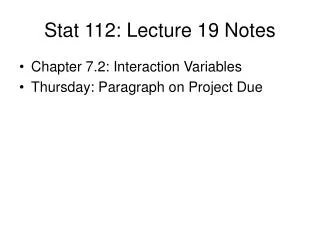
Regression Plot • The runs supervised by Alice appear abnormally time consuming. Bob has higher initial fixed setup costs than Carol (186.565>149.706) but has lower per unit production time (0.136<0.259).
Interaction Model • Interaction between run size and Manager: The effect on mean run time of increasing run size by one is different for different managers. • Is there strong evidence that there really is an interaction for the population? • Effect Test for Interaction: • Manager*Run Size Effect test tests null hypothesis that there is no interaction (effect on mean run time of increasing run size is same for all managers) vs. alternative hypothesis that there is an interaction between run size and managers. p-value =0.0333. Evidence that there is an interaction.
Interaction Profile Plot Lower left hand plot shows mean time for run vs. run size for the three managers Alice, Bob and Carol. Upper right hand plot shows mean run time for three managers for a low run size of 58 and a high run size of 345.
Interactions Involving Categorical Variables: General Approach • First fit model with an interaction between categorical explanatory variable and continuous explanatory variable. Use effect test on interaction to see if there is evidence of an interaction. • If there is evidence of an interaction (p-value <0.05 for effect test), use interaction model. • If there is not strong evidence of an interaction (p-value >0.05 for effect test), use model without interactions. The model without interactions is easier to interpret but should only be used if there is not strong evidence for interactions.
Example: A Sex Discrimination Lawsuit • Did a bank discriminatorily pay higher starting salaries to men than to women? Harris Trust and Savings Bank was sued by a group of female employees who accused the bank of paying lower starting salries to women. The data in harrisbank.JMP are the starting salaries for all 32 male and all 61 female skilled, entry-level clerical employees hired by the bank between 1969 and 1977, as well as the education levels and sex of the employees.
No evidence of an interaction between Sex and Education. Fit model without interactions.
Discrimination Case Regression Results • Strong evidence that there is a difference in the mean starting salaries of women and men of the same education level. • Estimated difference: Men have 345.904-(-345.904)=$691.81 higher mean starting salaries than women of the same education level. • 95% confidence interval for mean difference = (2*$214.55,2*$477.25)=($429.10,$854.50). • Bank’s defense: Omitted variable bias. Variables such as Seniority, Age, Experience also need to be controlled for.
Interpreting Coefficients When Y is Logged But Not X • Example: In an industrial laboratory, under uniform conditions, batches of electrical insulating fluid were subject to constant voltages until the insulating property of the fluids broke down. • Goal: Estimate E(Y|X), where Y=Breakdown Time, X=Voltage Level • The log Y transformation works well for this data:
Deciding on Variables • When we have many potential explanatory variables, how should we decide which to use? • Suppose our goal is to estimate the causal effect of a variable, controlling for all lurking variables (e.g., effect of pollution on mortality). Then it is best to include all possible lurking variables. Omitting variables, even if they do not appear significant leads to potential bias. • Suppose our goal is to understand the association of certain variable(s) with a response, holding fixed for certain other variables. We should think carefully about what variables we want to hold fixed.
Model Building for Prediction: General Principles • Include all variables that for substantive reasons, might be expected to be important in predicting the outcome. • For explanatory variables with large efects, consider their interactions as well. For each interaction considered, add the interaction if the p-value < 0.05 on the interaction term.
Excluding Variables From a Model • Should we ever drop a variable from a model? If there are many explanatory variables, then including variables that are not useful can worsen the estimates of the variables that are useful. • We suggest the following strategy: • If an explanatory variable is statistically significant (p-value < 0.05 for two sided test) and has the expected, then we should definitely keep it in the model. • If an explanatory variable is not statistically significant and has the expected sign, it is generally fine to keep the variable in the model. • If an explanatory variable is not statistically significant and does not have the expected sign and is not of primary interest in and of itself, we can consider removing it from the model. • If an explanatory variable is statistically significant but does not have the expected sign, then we should keep in the model, but think hard if the sign makes sense. Try to gather data on potential lurking variabls and include them in the analysis.
SAT Data • Y = Average score on 1982 SAT for the state. • Explanatory Variables: • X1=Takers (% of Total Eligible Students in the state who took the exam). • X2=Income (Median Income of Families of Test Takers) • X3=Years (Average Number of Years That Test Takers Had Formal Studies in Social Sciences, Natural Sciences and Humanities) • X4=Public (Percentage of Test Takers who attend public schools) • X5=Expend (Total State Expenditure on Secondary Schools, expressed in hundreds of dollars per student) • X6=Rank (Median percentile ranking of test takers within their secondary classes)
Expected Signs • X1=Takers (% of Total Eligible Students in the state who took the exam) (Expected sign: -) • X2=Income (Median Income of Families of Test Takers) (Expected sign: +) • X3=Years (Average Number of Years That Test Takers Had Formal Studies in Social Sciences, Natural Sciences and Humanities) (Expected sign: +) • X4=Public (Percentage of Test Takers who attend public schools) (Expected sign: -) • X5=Expend (Total State Expenditure on Secondary Schools, expressed in hundreds of dollars per student) (Expected sign: +) • X6=Rank (Median percentile ranking of test takers within their secondary classes) (Expected sign: +)