Stat 112 Notes 11
Stat 112 Notes 11. Today: Fitting Curvilinear Relationships (Chapter 5) Homework 3 due Friday. I will e-mail Homework 4 tonight, but it will not be due for two weeks (October 26 th ). Curvilinear Relationships . Relationship between Y and X is curvilinear if E(Y|X) is not a straight line.


Stat 112 Notes 11
E N D
Presentation Transcript
Stat 112 Notes 11 • Today: • Fitting Curvilinear Relationships (Chapter 5) • Homework 3 due Friday. • I will e-mail Homework 4 tonight, but it will not be due for two weeks (October 26th).
Curvilinear Relationships • Relationship between Y and X is curvilinear if E(Y|X) is not a straight line. • Linearity for simple linear regression model is violated for a curvilinear relationship. • Approaches to estimating E(Y|X) for a curvilinear relationship • Polynomial Regression • Transformations
Transformations • Curvilinear relationship: E(Y|X) is not a straight line. • Another approach to fitting curvilinear relationships is to transform Y or x. • Transformations: Perhaps E(f(Y)|g(X)) is a straight line, where f(Y) and g(X) are transformations of Y and X, and a simple linear regression model holds for the response variable f(Y) and explanatory variable g(X).
Curvilinear Relationship Y=Life Expectancy in 1999 X=Per Capita GDP (in US Dollars) in 1999 Data in gdplife.JMP Linearity assumption of simple linear regression is clearly violated. The increase in mean life expectancy for each additional dollar of GDP is less for large GDPs than Small GDPs. Decreasing returns to increases in GDP.
The mean of Life Expectancy | Log Per Capita appears to be approximately a straight line.
How do we use the transformation? • Testing for association between Y and X: If the simple linear regression model holds for f(Y) and g(X), then Y and X are associated if and only if the slope in the regression of f(Y) and g(X) does not equal zero. P-value for test that slope is zero is <.0001: Strong evidence that per capita GDP and life expectancy are associated. • Prediction and mean response: What would you predict the life expectancy to be for a country with a per capita GDP of $20,000?
How do we choose a transformation? • Tukey’s Bulging Rule. • See Handout. • Match curvature in data to the shape of one of the curves drawn in the four quadrants of the figure in the handout. Then use the associated transformations, selecting one for either X, Y or both.
Transformations in JMP • Use Tukey’s Bulging rule (see handout) to determine transformations which might help. • After Fit Y by X, click red triangle next to Bivariate Fit and click Fit Special. Experiment with transformations suggested by Tukey’s Bulging rule. • Make residual plots of the residuals for transformed model vs. the original X by clicking red triangle next to Transformed Fit to … and clicking plot residuals. Choose transformations which make the residual plot have no pattern in the mean of the residuals vs. X. • Compare different transformations by looking for transformation with smallest root mean square error on original y-scale. If using a transformation that involves transforming y, look at root mean square error for fit measured on original scale.
` By looking at the root mean square error on the original y-scale, we see that all of the transformations improve upon the untransformed model and that the transformation to log x is by far the best.
The transformation to Log X appears to have mostly removed a trend in the mean of the residuals. This means that . There is still a problem of nonconstant variance.
Comparing models for curvilinear relationships • In comparing two transformations, use transformation with lower RMSE, using the fit measured on the original scale if y was transformed on the original y-scale • In comparing transformations to polynomial regression models, compare RMSE of best transformation to best polynomial regression model (selected using the criterion from Note 10). • If the transfomation’s RMSE is close to (e.g., within 1%) but not as small as the polynomial regression’s, it is still reasonable to use the transformation on the grounds of parsimony.
Transformations and Polynomial Regression for Display.JMP Fourth order polynomial is the best polynomial regression model using the criterion on slide 10 Fourth order polynomial is the best model – it has the smallest RMSE by a considerable amount (more than 1% advantage over best transformation of 1/x.
Log Transformation of Both X and Y variables • It is sometimes useful to transform both the X and Y variables. • A particularly common transformation is to transform X to log(X) and Y to log(Y)
Evaluating Transformed Y Variable Models The log-log transformation provides slightly better predictions than the simple linear regression Model.
Another Example of Transformations: Y=Count of tree seeds, X= weight of tree
By looking at the root mean square error on the original y-scale, we see that Both of the transformations improve upon the untransformed model and that the transformation to log y and log x is by far the best.
Prediction using the log y/log x transformation • What is the predicted seed count of a tree that weights 50 mg? • Math trick: exp{log(y)}=y (Remember by log, we always mean the natural log, ln), i.e.,