Download
1 / 19
190 likes | 387 Vues
Multi-decadal Coupled Sea-ice/Ocean Numerical Simulations of the Bering Sea. Kate Hedstrom, ARSC/UAF Enrique Curchitser, LDEO Al Hermann, PMEL January, 2006. Bering Sea. Motivation and background Bering sea model implementation Results: Circulation Sea-ice cover

E N D
Multi-decadal Coupled Sea-ice/Ocean Numerical Simulations of the Bering Sea Kate Hedstrom, ARSC/UAF Enrique Curchitser, LDEO Al Hermann, PMEL January, 2006
Bering Sea • Motivation and background • Bering sea model implementation • Results: • Circulation • Sea-ice cover • Interannual variability and trends • Conclusions and future work
Motivation • A yardstick for climate change (sea ice) • High primary productivity • Significant commercial fisheries (Pollock) • Comparison with other sub-Arctic seas (e.g., Barents)
The Model • ROMS ocean • F90 • Now with an adjoint and tangent linear for data assimilation • Ice model from Paul Budgell • EVP dynamics (Arakawa C grid) • Mellor-Kantha thermodynamics • Oceanic molecular sublayer under the ice for improved behavior
10 km average horizontal resolution Run1: 30 vertical layers IC’s and BC’s from NPac Daily fluxes from NCEP hindcast (modified) 1996-2002, 1960-1970 Run2: 42 vertical layers IC’s and BC’s from CCSM (POP) Six-hourly fluxes from CCSM hindcast 1958-2000+, up to 1974 so far NEP Implementation
Sea ice concentration: January 1996 ROMS - NCEP SSM/I+
Sea ice concentration: January 1997 ROMS - Run 1 SSM/I+
Sea ice concentration: January 1998 ROMS - Run 1 SSM/I+
Lessons from a “bad” simulation: The global warming scenario NCEP (tweaked) NCEP
ROMS - NCEP ROMS - CCSM Sea Surface Temperature
ROMS - NCEP ROMS - CCSM Sea-ice Concentration: April 1966
ROMS - NCEP ROMS - CCSM Sea-ice Concentration: April 1969
ROMS - NCEP ROMS - CCSM Sea-ice Concentration: April 1963
Future Plans • Finish the 10 km run driven by CCSM forcing • Run on the 4 km grid • Four tidal constituents from Mike Forman • Closer to eddy resolving • Estimate 200 hours/year on 48 pwr4 processors • Add an ecosystem model (and modeler)
Conclusions • The model reproduces the seasonal and interannual variability in the sea-ice conditions as well as the major circulation features • The CCSM forcing fields are a significant improvement: • Higher time resolution • No hack to the heat fluxes • We hope to use these simulations to improve our understanding of the circulation and ecosystem in the Bering Sea