FAST TCP: Motivation, Architecture, Algorithms, Performance
330 likes | 546 Vues
Cheng Jin David Wei Steven Low. FAST TCP: Motivation, Architecture, Algorithms, Performance. http:// netlab.caltech.edu. Difficulties at large window. Equilibrium problem Packet level : AI too slow, MD too drastic. Flow level : requires very small loss probability. Dynamic problem

FAST TCP: Motivation, Architecture, Algorithms, Performance
E N D
Presentation Transcript
Cheng Jin David Wei Steven Low FAST TCP:Motivation, Architecture, Algorithms, Performance http://netlab.caltech.edu
Difficulties at large window • Equilibrium problem • Packet level: AI too slow, MD too drastic. • Flow level: requires very small loss probability. • Dynamic problem • Packet level: must oscillate on a binary signal. • Flow level: unstable at large window.
Problem: binary signal TCP oscillation
Solution: multibit signal FAST stabilized
Queueing Delay in FAST Queueing delay is not used to avoid loss Queueing delay defines a target number of packets () to be buffered for each flow Queueing delay allows FAST to estimate the distance from the target
Problem: no target • Reno:AIMD (1, 0.5) ACK: W W + 1/W Loss: W W – 0.5W • HSTCP:AIMD (a(w), b(w)) ACK: W W + a(w)/W Loss: W W – b(w)W • STCP:MIMD (1/100, 1/8) ACK: W W + 0.01 Loss: W W – 0.125W
Solution: estimate target • FAST FAST Conv Slow Start Equil Loss Rec Scalable to anyw*
Implementation Strategy • Commonflow level dynamics window adjustment control gain flow level goal • Small adjustment when close, large far away • Need to estimate how far current state is from tarqet • Scalable • Queueing delay easier to estimate compared with extremely small loss probability =
Window Control Algorithm • RTT: exponential moving average with weight of min {1/8, 3/cwnd} • baseRTT: latency, or minimum RTT • determines fairness and convergence rate
FAST and Other DCAs FAST is one implementation within the more general primal-dual framework Queueing delay is used as an explicit feedback from the network FAST does not use queueing delay to predict or avoid packet losses FAST may use other forms of price in the future when they become available
Architecture Each component • designed independently • upgraded asynchronously Data Control Window Control Burstiness Control Estimation TCP Protocol Processing
Experiments In-house dummynet testbed PlanetLab Internet experiments Internet2 backbone experiments ns-2 simulations
Dummynet Setup • Single bottleneck link, multiple path latencies • Iperf for memory-to-memory transfers • Intra-protocol testings • Dynamic network scenarios • Instrumentation on the sender and the router
What Have We Learnt? FAST is reasonable under normal network conditions Well-known scenarios where FAST doesn’t perform well Network behavior is important Dynamic scenarios are important Host implementation (Linux) also important
Dynamic sharing: 3 flows FAST Linux Steady throughput HSTCP STCP
Aggregate Throughput Dummynet: cap = 800Mbps; delay = 50-200ms; #flows = 1-14; 29 expts Ideal CDF large windows
Stability Dummynet: cap = 800Mbps; delay = 50-200ms; #flows = 1-14; 29 expts stable under diverse scenarios
Fairness Dummynet: cap = 800Mbps; delay = 50-200ms; #flows = 1-14; 29 expts Reno and HSTCP have similar fairness
Room for mice ! 30min queue FAST Linux loss throughput HSTCP STCP HSTCP
Known Issues Network latency estimation route changes, dynamic sharing does not upset stability Small network buffer at least like TCP Reno adapt on slow timescale, but how? TCP-friendliness friendly at least at small window how to dynamically tune friendliness? Reverse path congestion
Acknowledgments • Caltech • Bunn, Choe, Doyle, Newman, Ravot, Singh, J. Wang • UCLA • Paganini, Z. Wang • CERN • Martin • SLAC • Cottrell • Internet2 • Almes, Shalunov • Cisco • Aiken, Doraiswami, Yip • Level(3) • Fernes • LANL • Wu
http://netlab.caltech.edu/FAST • FAST TCP: motivation, architecture, algorithms, performance. IEEE Infocom 2004 • Code reorganization, ready for integration with web100. • b-release: summer 2004 Inquiry:fast-support@cs.caltech.edu
Backward Queueing Delay IIBartek Wydrowski 1 fw flow 1 bk flow 2 fw flows 2 bk flows 2 fw flows 1 bk flows
PlanetLab Internet Experiment Jayaraman & Wydrowski Throughput v.s. loss and delay qualitatively similar results FAST saw higher loss due to large alpha value
Linux Related Issues Complicated state transition Linux TCP kernel documentation Netdev implementation and NAPI frequent delays between dev and TCP layers Linux loss recovery too many acks during fast recovery high CPU overhead per SACK very long recovery times Scalable TCP and H-TCP offer enhancements
TCP/AQM AQM: • DropTail • RED • REM/PI • AVQ TCP: • Reno • Vegas • FAST pl(t) xi(t) • Congestion control has two components • TCP: adjusts rate according to congestion • AQM: feeds back congestion based on utilization • Distributed feed-back system • equilibrium and stability properties determine system performance
Optimization Model Network bandwidth allocation as utility maximization Optimization problem Primal-dual components x(t+1) = F(q(t), x(t)) Source p(t+1) = G(y(t), p(t)) Link U ( x ) max s s x 0 s s subject to y c , l L l l
Network Model Rf(s) F1 G1 Network TCP AQM FN GL q p Rb(s) x y • Components: TCP and AQM algorithms, and routing matrices • Each TCP source sees an aggregate price, q • Each link sees an aggregate incoming rate
Packet Level • Reno AIMD(1, 0.5) • HSTCP AIMD(a(w), b(w)) • STCP MIMD(a, b) • FAST ACK: W W + 1/W Loss: W W – 0.5 W ACK: W W + a(w)/W Loss: W W – b(w) W ACK: W W + 0.01 Loss: W W – 0.125 W