Download
1 / 32
320 likes | 532 Vues
MAE6291 Class 2 ELISA (Enzyme-linked immune sandwich assay) Binding kinetics and equilibrium Brownian motion and diffusion Surface plasmon resonance (SPR) sensors. monoclonal or polyclonal binds diff. epitope than capture ab may be directly conj. to enzyme

E N D
MAE6291 Class 2 ELISA (Enzyme-linked immune sandwich assay) Binding kinetics and equilibrium Brownian motion and diffusion Surface plasmon resonance (SPR) sensors
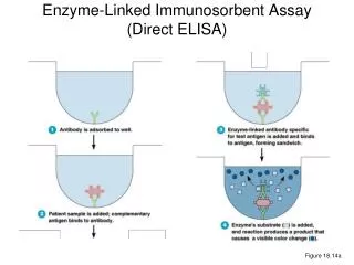
monoclonal or polyclonal binds diff. epitope than capture ab may be directly conj. to enzyme or enzyme introduced via 3rdAb that binds detection Ab or enzyme-avidin conjugate if detection Abbiotinylated “receptor” Typical ELISA format monoclonal or polyclonal usually immobilized on plate by commercial supplier could be microbial antigen if goal is to detect antibodies to it then detection ab is anti-IgG
Typical protocol Add sample in ~200ml, incubate ~1.5h (why so long?), wash Add 20 Ab coupled to enzyme (e.g HRP).incubate 1.5h, wash Add enz. substrate (e.g. tetramethylbenzene) Incubate 30min (in dark) Add stop solution (H2SO4) (why?), read OD (within 30min) Analyte with know concentration serially diluted in some wells to compare intensities to that of sample Result: analyte conc. in sample
What determines sensitivity, incubation times?
Reaction (receptor binding) kinetics Let bm = total receptor conc. on sensor surface [moles/area] b(t) = conc of receptors that have bound analyte at time t Assume analytebinds receptor at rate ~ freeanalyteconc., c0,* free receptor conc., [bm – b(t)] and dissociates from receptor at rate ~b(t) db(t)/dt= konc0 [bm – b(t)] – koffb(t) kon and koff are constants
db(t)/dt= konc0 [bm – b(t)] – koffb(t) Interpretation of binding constants kon = av. # “binding” collisions/s each receptor molecule makes with an analyte molecule when analyteconc = 1 in whatever units you use, e.g. #/m3 or “molar”, M, moles/l Units of konare #/conc.*time, e.g. M-1s-1 koff = rate each receptor-analyte complex dissociates in #/s Define KD=koff/konUnits of KD are conc., e.g. M
db(t)/dt= konc0 [bm – b(t)] – koffb(t) Solution: b(t)/bm= fraction of receptors with analyte= A(1-e-Bt) where A = [c0/KD /(1 + c0/KD)] and B = konc0 + koff A = c0/KD /(1 + c0/KD) b(t)/bm time t = 1/B = koff-1/(1+c0/KD)
c0/KD /(1 + c0/KD) b(t)/bm natural to measure concentrations in units of KD when c0 = KD, half of receptors have bound analyte c0 >> KD, fraction of receptors with analyte -> 1 c0 << KD, most receptors are free typical values kon~ 106/Ms ( =10-21m3/s) fairly constant koff~ 1/s to 1/103s (varies a lot) KD~mM (weak) to nM (tight binding) Note smaller KD <-> tighter binding (slower koff) time t = koff-1/(1 + c0 /KD)
Receptor and analyte are interchangeable in this model Excess receptor drives binding of analyte Excess analyte drives binding of receptor Model assumes mixing keeps concentration uniform c0 = freeanalyteconc, lower than initial concci in ELISA Model describes behavior of large # of molecules; when only a few analyte molecules/sensor, need to consider stochastic issues more carefully More detailed analysis takes into account depletion of analyte in region just above receptor due to its binding and flux if convective flow (next week)
Details of some example ELISA assays http://www.bioxys.com/i_Zeptometrix/0801111.htm http://www.ebioscience.com/human-il-1-beta-high-sensitivity-elisa-kit.htm suppose kon= 106/Ms, koff = 10-3/s, KD = 10-9M c0 ~ 0.1pM = 107/well (100ml) << KD bm~ 1/(10nm)2= 1011/3mm well What fraction of receptors bind analyte? How long to reach equilibrium? 10 nm Assay takes hours bec. of equil. times Sensitivity limited by # enz. req. to generate signal and “noise” due to non-specific sticking (of detection Ab and subsequent reagents) Reagent costs <1$/well; ~$100/plate; OD plate reader ~$10-30K
What is sensitivity of high end ELISA? How many molecules in 100ml sample @ 0.5pg/ml If KD=nM and 1011 capture Abs/well, what fraction of analyte is bound? Hint: switch roles of anal. and receptor in formula for fx bound * Analyte MW = 20kDa (20,000g/mole)
Diffusion and Brownian motion • Why do molecules diffuse? • How far do they go (on average) in time t? • Let <x2(t)> = av. displacement2 of molecule after time t • Why talk in terms of <x2(t)>? What is <x(t)>? • <x2(t)> =~ t Why not ~t2? They keep changing directions. • In 1-d, suppose molecule moves randomly +e every t sec • <(xnt)2> = <(x(n-1)t +e)2> = <(x(n-1)t)2 + 2x(n-1)te+ e2> = ne2 • since n = t/t, <x2(t)> = (e2/t)t =Dtwhere D is diff. const. • Note D=e2/thas units of m2/s
Deep connection between D and viscous drag: both are due to bombardment by adj. molecules In laminar flow, drag force on sphere radius r Fdrag = gv where g = 6phr Stokes law h=viscosity, 10-3 Ns/m2 in water v = velocity of sphere Einstein relation: Dg = kBT = 4x10-21J at R.T. Utility: If you know r, you know D = kBT/6phr mol. with r~2nm has D = 4x10-21/.04x 10-9 = 10-10m2/s virus with r~200nm has D = 10-12m2/s
About how long does it take a 2nm molecule to diffuse 3mm? (approx. distance to surface in microtiter plate well)? t = x2/6D in 3dimensions = 9x10⁻⁶/6x10-10 = 104s (hours!) twice dimension # why ELISA takes so long Bulk flow of molecules down a concentration gradient is due to diffusion Fick’s Law: flux j D (# molecules crossing unit area per s) = D dc/dx check that units agree! this becomes important for SPR sensors
Surface plasmon resonance (SPR) sensors Like real-time immune capture assay without need for second Ab Sensing principle – light incident on glass surface > critical angle is totally reflected; if glass has thin metallic coating, evanescent wave in metal polarized in plane of incidence canexcite coherent movement of electrons on metal surface when resonance condition kx = ksp is met
Surface Plasmon Resonance – prism configuration 2 q Since kx = (w/c) ng sin q = ksp, surface plasmon excited at particular incidence angle qr -> decrease in reflection intensity ksp very sensitive to n2~ mass bound to metal surface To first order, Dqr ~ Dm
How sensitive is Dqrto Dm? Typical sensitivity limit is ~1pg (~107 molecules for MW 105) in sensor area 1mm2 (roughly comparable to ELISA); this is equiv. to covering ~ 1/1000th of surface Less sensitive per bound molecule when tgt is small (signal ~mass bound) but still can be used to study protein-drug interactions Major advantages cf to ELISA real time results, don’t need label, more automatable get kinetic parameters kon, koff, KD, and bm as well as c0 Major disadvantage – cost ~$100K/machine + exp. chips
Lots of info available on web and from vendors, e.g. Biacore, now part of GE http://www.biacore.com/lifesciences/technology/introduction/following_interaction/index.html http://www.biacore.com/lifesciences/technology/introduction/data_interaction/index.html Note SPR facilitates depositing your own receptors http://www.protein.iastate.edu/seminar/BIACore/ TechnologyNotes/TechnologyNote1.pdf http://www.bama.ua.edu/~chem/seminars/ student_seminars/fall08/f08-papers/ bokatzian-johnson-sem.pdf http://www.biosensingusa.com/Application101.html
Characteristic SPR binding curves Conc that -> half max binding = KD Flow in analyte Flow in buffer (analyte elutes) charact. off time = 1/koff 1RU=10-4 degrees analyte conc. nM Can you estimate 1/koff from these curves? Can you estimate conc. that gives half max binding? Do they wait long enough to reach binding equilibrium?
Are binding kinetics influenced by flow rate, channel dimensions, sensor dimensions? E.g. as molecules adsorb to surface, are they depleted from region just above surface? What does this do to concentration near surface? To binding rate? # molecules that bind/s = koncs [bm-b(t)] Does incoming flow keep cs = c0? Need more detailed model of mass transport to extract KD, kon from raw data = next week’s topic
Example – kinetic constants extracted from SPR data for binding of various engineered, antibody-like molecules to their targets Note ~106/Ms ~1/1000s ~nM
SPR is work-horse for analysis of protein interactions in biochemistry labs/ pharmaceutical industry Does it need to be so expensive? Texas Instruments’ SPR chip - SPREETA Sensors and Actuators B 91 (2003) 266–274 Could you put one in cell phone?
Other questions What limits sensitivity of SPR? What determines width of resonance? What is effect of spatial inhomogeneity of bound analyte on molecular scale? What is effect of distance of analyte from metal surface?
Summary – most assays we’ll consider involve analyte binding to surface, with direct detection (“label-free”) due to effect on some physical phenomenon – e.g. surface plasmon resonance frequency, or detection via attachment of a “label” that provides a signal, e.g. enzyme that generates dye in ELISA
Specificity for particular analyte (essential in biosensors because almost always dealing with very complex mixtures of related molecules) comes from capture molecules (e.g. antibody, compl. DNA) This means interactions with capture molecules are crucial b(t)/bm = [c0/KD /(1 + c0/KD)][1-exp-(konc0 + koff)t] (c0/KD)/(1 + c0/KD) b(t)/bm time t = 1/(konc0 + koff)
Sensitivity usually not better than 107 molecules [pM] for conventional sensors, but coming down to 1 molecule for new technologies (major subject of course) Assay times affected by mass transport kinetics plus diffusion plus kinetics of binding to capture molecules – topic for next week
Intro to next week’s paper – mass transport limits for standard format biosensors sensor surface Sensor kinetics depends on 3 main processes: sample flow rate, diffusion of molecules to sensor surface, binding kinetics
Good matching of rates of these processes important for sensor function Binding of target molecules to sensor surface depletes region near surface of targets (lowers cs), slows response Color shows depletion of targets (blue) in regions of flow cell as function of time if no flow analyteconc scale
Flow restores target molecules to depleted regions but very rapid flow (in e) -> many molecules whiz by before they can diffuse to surface analyteconc
Depletion region dimensions depend on D, L, H, flow rate Simple ratios of these parameters, PeH and PeS, determine if sensor is operating in regime that looks like c versus e What does concentration profile look like if you wait for equilibrium?
Another ratio, Da, determines if time to reach steady-state is determined mainly by chemical reaction trxn = koff-1/(1 + c0 /KD) or strongly affected by diffusion, geometry and receptor density teq = Datrxnwhere Da is function of D, L, H, kon and bm This analysis especially important when pushing sensitivity to detect very low conc. targets
Divide segments of Manalis paper for student presentations Fig. 1 + summarize relations between flow rate, speed as function of height, pressure, from rest of paper Fig. 2 – depletion region dimensions as function of time in absence of flow Fig. 3. – intitial (quasi-steady state) depletion region dimensions given flow, Peclet numbers Fig. 4. and Box 3 – 2 particluar sensors Fig. 5. and Damkohler # Box 2 – low conc. trade-offs