Download
1 / 34
340 likes | 363 Vues
Explore the Semi-Lagrangian approximation methods for solving time-dependent Navier-Stokes equations using Finite Element Method, with emphasis on advection derivative accuracy. Learn about interpolation stability and conservation laws in computational fluid dynamics.

E N D
Semi-Lagrangian Approximation in the Time-Dependent Navier-Stokes Equations Vladimir V. Shaydurov Institute of Computational Modeling of Siberian Branch of Russian Academy of Sciences, Krasnoyarsk Beihang University, Beijing shaidurov04@mail.ru in cooperation with G. Shchepanovskaya and M. Yakubovich
Contents • Convection-diffusion equations: • Modified method of characteristics. • Conservation law of mass: • Approximation in norm. • Finite element method: • Approximation in norm.
Pironneau O. (1982): Method of characteristics The main feature of several semi-Lagrangian approaches consists in approximation ofadvection members as one “slant”(substantial or Lagrangian) derivative in the direction of vector
Pointwise approach in convection-diffusion equation The equation with this right-hand side is self-adjoint.
Approximation of slant derivative Apply finite element method at the time level and use appropriate quadrature formulas for the lumping effect Two ways for approximation of slant derivative 1. Approximation along vector 2. Approximation along characteristics (trajectory)
Approximation of substantial derivative along trajectory Solution smoothness usually is better along trajectory Asymptotically both way have the same first order of approximation
Finite element formulation at time level Intermediate finite element formulation Final formulation
Interpolation-1 Stability in norm: Chen H., Lin Q., Shaidurov V.V., Zhou J. (2011), …
Interpolation-1 Stability in norm and conservation law: impact of four neighboring points into the weight of
Solving two problems with the first and second order of accuracy
Navier-Stokes equations In the cylinder we write 4 equations in unknowns
Boundary conditions at subsonic part of computational boundary a wake
Direct approximation of Curvilinear hexahedron V: Trajectories:
Due to Gauss-Ostrogradskii Theorem: Approximation of curvilinear quadrangle Q:
Gauss-Ostrogradskii Theorem in the case of boundary conditions:
Supersonic flow around wedge M=4, Re=2000 angle of the wedge β ≈ 53.1º, angle of attack = 0º Density and longitudinal velocity at t = 8 Density and longitudinal velocity at t = 20
Supersonic flow around wedge for nonzero angle of attack M=4, Re=2000 angle of the wedge β= 53.1º, angle of attack = 5º Density and longitudinal velocity at t = 6 Density and longitudinal velocity at t = 8
Density and longitudinal velocity at t = 10 Density and longitudinal velocity at t = 20
Density M=4, Re=2000 Angle of the wedgeβ ≈ 53.1° Longitudinal velocity
Conclusion • Conservation of full energy (kinetic + inner) • Approximation of advection derivatives in the frame of finite element method without artificial tricks • The absence of Courant-Friedrichs-Lewy restriction on the relation between temporal and spatial meshsizes • Discretization matrices at each time level have better properties • The better smooth properties and the better approximation along trajectories