Download
1 / 34
340 likes | 732 Vues
Human Visual Perception and Retinal Diseases. Carmen Alina Lupaşcu Dipartimento di Matematica e Informatica Università degli Studi di Palermo. Structure of the human eye. The human visual system has the ability to assimilate information from visible light which reaches the eye. .

E N D
Human Visual Perception and Retinal Diseases Carmen Alina Lupaşcu Dipartimento di Matematica e Informatica Università degli Studi di Palermo June 8, 2010 Gjøvik, Norway
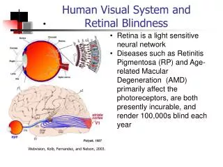
Structure of the human eye The human visual system has the ability to assimilate information from visible light which reaches the eye. The human eye has a spherical shape and it is wrapped in three distinct layers of tissue: • the outer layer – the sclerotic coat; • the middle layer – the choroid coat; • the inner layer – the retina. Movement of the eyeball produces two slightly differing views of the same scene which our brain is able to fuse into a single, three-dimensional image. June 8, 2010 Gjøvik, Norway 2
Structure of the human retina The retina - capture light rays and convert them into electrical impulses that travel along the optic nerve to the brain where they are turned into images. The macula - small part of the retina responsible for detailed central vision (such as reading). The fovea - the center of the macula. The optic nerve – transmits electrical impulses from the retina to the brain. The optic disc is the point where the optic nerve enters the retina and it is not sensitive to light. The blood vessels of the retina radiate from the center of the optic nerve. June 8, 2010 Gjøvik, Norway 3
Retinal pathologies • Diseases of the retina can be responsible for partial or total loss of vision. Some retinal pathologies are caused also by the presence of other diseases such as diabetes. • The symptoms presented by patients affected by retinal diseasesmaybe: • peripheral vision or side vision deteriorated - in the presence of glaucoma (disease that causes injury to the eye’s optic nerve); Normal vision Same scene viewedby a personwith glaucoma June 8, 2010 Gjøvik, Norway 4
reduced visual acuity. Blurring of vision may affect sight in the presence of diseases such as papilledema (optic disc swelling due to • intra cranial pressure) or age-related macular • degeneration AMD (is a disease associated with aging that • slowly destroys central vision which is needed for seeing • objectsclearly); • poor color vision. Patients with optic atrophy (disease which affects the optic nerve by loosing part of optic disc nerve fibers) may have difficulties with color vision. Color vision is perceived mainly by the macula. Thus any pathology affecting the macula may cause also difficulties with color vision; June 8, 2010 Gjøvik, Norway 5
obscured visual field. Vision may be obstructed by spots of blood caused by swelled and leaky blood vessels of the retina like in the case of diabeticretinopathy. Normal vision Same scene viewed by a person with diabetic retinopathy • image distortion. Straight lines may appear broken or distorted in the presence of macular pathologies, like for example AMD. Scene viewedby a personwith macular disease June 8, 2010 Gjøvik, Norway 6
Types of retinal photography Fluorescein angiography A camera equipped with special filters that highlight the dye is used to photograph the fluorescein as it circulates though the retinal blood vessels. If there are any circulation problems, swelling, leaking or abnormal blood vessels, the dye and its patterns will reveal these in the photographs. Digital retinal fundus photography.A fundus camera is a type of "ophthalmoscope" or “funduscope". Some of the retinal cameras available require pupillary dilation, while others do not. The ones requiring pupillary dilation are called mydriatic cameras, the others non-mydriatic cameras. June 8, 2010 Gjøvik, Norway 7
Fluorescein angiograms Courtesy of ClinicaOculistica, PoliclinicoUniversitario Paolo Giaccone, Palermo, Italy June 8, 2010 Gjøvik, Norway 8
Normal digital retinal images Healthy vessels Healthy macula Healthy optic disc http://www.isi.uu.nl/Research/Databases/DRIVE/ June 8, 2010 Gjøvik, Norway 9
Abnormal digital retinal images D U E T O D I S E A S E S Optic disc disease (optic pit) Optic disc disease (optic disc hypoplasia) http://www.revoptom.com/HANDBOOK/ June 8, 2010 Gjøvik, Norway 10
Abnormal digital retinal images D U E T O P H O T O G R A P H I C Q U A LI T Y Uneven illumination Dust and dirt artifacts http://eyephoto.ophth.wisc.edu/ResearchAreas/Hypertension/LBox/LTBXPROT_995.html June 8, 2010 Gjøvik, Norway 11
Digital image analysis Advantages: • the retina can be directly analyzed non-invasively in vivo • possibility to analyze a large number of images with time and cost savings • objective measurements • improved repeatability Disadvantages: • image quality (may be improved using preprocessing techniques) June 8, 2010 Gjøvik, Norway 12
Automated optic disc detection Initial point – the center of mass of the region with maximum intensity within the green plane (black ’+’) Points of interest – 3 for each 45° in counter-clockwise direction starting from the initial point(black ’.’) in the left image; excluded points marked with a dark circle (’o’) in the right image June 8, 2010 Gjøvik, Norway 13
From the set of the remaining points of interest, all possible sets of three such points were formed. If we have such a set of points, through these points one circle passes. All three points from the set are different and in one set there are not two points from the same ’direction’, thus we are sure that the points are not all collinear. • For each circle we consider the grey level of the pixels inside the disk and on the circumference. For this region we compute some descriptors of texture based on the intensity histogram of the region, in order to describe better the circle and in order to choose the best circle that fits the OD. • uniformity < mean(uniformity all circles) entropy > mean(entropy all circles) third moment > mean(third moment all circles) smoothness > mean(smoothness all circles) 315 183 88 913 575 June 8, 2010 Gjøvik, Norway 14
Each remained circle is mapped using the bilinear filtering into the polar coordinates space. Mapping images For the circle which best fits the OD The circle which best fits the OD A circle which doesn’t fit the OD For a circle which doesn’t fit the OD June 8, 2010 Gjøvik, Norway 15
In only one central strip of the mapping image we look for the maximum derivatives in the y direction. The regression line that best fits the set of the derivatives The maximum derivatives in the y direction The strip of the mapping image For the circle which best fits the OD For the circle which best fits the OD For a circle which best fits the OD For a circle which doesn’t fit the OD For a circle which doesn’t fit the OD For the circle which doesn’t fit the OD • To the set of the points of maximum derivatives in the y direction we apply the linear least squares fitting technique (linear regression). We try to find the best fitting straight line passing through the set of points described above. In order to quantify the quality of the fitting to the original data we compute the correlation coefficient. June 8, 2010 Gjøvik, Norway 16
In order to compute the correlation coefficient of a set of n data points (xi; yi), we first consider the sum of squared values ssxx, ssxy and ssyy about their respective means, and where and . June 8, 2010 Gjøvik, Norway 17
The correlation coefficient is • The equation of the regression line will be where and • We expect to have a correlation coefficient big (close to 1) for the circle that best fits the OD (as the maximum derivatives in the y direction are expected to be at the OD boundary). • The circle that best fits the OD is chosen as the circle with the maximum correlation coefficient associated. June 8, 2010 Gjøvik, Norway 18
Evaluation method • In order to evaluate if the circle obtained by our algorithm fits the OD as good as the ground truth (set manually by an ophthalmologist) we consider the ratio where GT is the ground truth circle and C is the circle obtained by the methodology. • A ratio S => 0,7 indicates an excellent result (E), 0,5 <= S < 0,7 denotes a good (G) result which requires improvement and S < 0,5 a fair (F) result. We have two bad results (B) because of the wrong positioning of the initial point (the initial point was chosen as the center of mass of the pixels with the maximum intensity within the green plane of the image). In these bad quality images the initial point is not within the OD area and that’s why we have false detection of the OD. • For the best circle which fits the OD, we consider successful a circle which has associated a ratio S >= 0,5, hence our algorithm achieved a success rate of 70%. June 8, 2010 Gjøvik, Norway 19
Examples of detected optic discs. The detected optic disc (bright contour) overlaps the ground truth (dark contour). E X C E L L E N T R E S U L T June 8, 2010 Gjøvik, Norway 20
Examples of detected optic discs. The detected optic disc (bright contour) overlaps the ground truth (dark contour). G O O D R E S U L T Ground truth Detected OD June 8, 2010 Gjøvik, Norway 21
Examples of detected optic discs. The detected optic disc (bright contour) overlaps the ground truth (dark contour). F A I R R E S U L T Ground truth Detected OD June 8, 2010 Gjøvik, Norway 22
Results • Advantages of the methodology: • lack of training • wedon’t use Hough transform for detecting the best circle that fits the OD and this because we don’t want to fix a priori a range for the radius of the circle or to fix a threshold value on the number of pixels of the circle • Improvements that can be made: • the way we choose the initial point. This point is chosen as the center of mass of the pixels with the maximum intensity within the green plane. In some bad quality images this choice cause a false detection of the OD. • Success rate: • 40 testing images (DRIVE database http://www.isi.uu.nl/Research/Databases/DRIVE/) • 95% for the localization of the OD position • 70% for the circle that is best fitting the OD June 8, 2010 Gjøvik, Norway 23
Retinal vessel segmentation Feature AdaBoost Classification (FABC) FABC trains an AdaBoost classifier with manually labeled images. After the classifier is trained, it is applied to classify pixels as vessel or non-vessel in images not included in the training set. FEATURE VECTOR Features are extracted from the green plane of the retinal images. The total number of features composing the feature vector at each image pixel is 41. Four scales are used to detect vessels of different width: √2, 2, 2√2 and 4. Sample selection • FABC(w/o feature selection) • leave-one-out tests using all 40 images in the DRIVE database • 864,697/39 pixels from each image, keeping the same proportion as in the ground-truth image between vessel and non-vessel pixels. • The sample size was computed with a Z-test, considering a confidence level of 95% and a margin of error of 0.1%. June 8, 2010 Gjøvik, Norway 24
Outline of the methodology June 8, 2010 Gjøvik, Norway 25
AdaBoost algorithm Is an iterative boosting algorithm constructing a strong classifier as a linear combination of weak classifiers. Input: is a n-dimensional feature vector (here n=41) labels T=100 how many times the AdaBoost growing classifier runs when t=1 (the round index) D1(i)=1/m, Dt(i) denotes the weight of the distribution Task: find a weak hypothesis suitable for the distribution Dt(i) (the weak learner searches for by checking all possible thresholds for all features) weak learner algorithm for a fixed feature j (j=1,…,n) June 8, 2010 Gjøvik, Norway 26
Evaluation method The performance of the binary classifier are measured using Receiver Operating Characteristic (ROC) curves. ROC curves are represented by plotting true positive fractions versus false positive fractions as the discriminating threshold of the AdaBoost algorithm is varied. The area under the ROC curve (Az) measures discrimination, that is the ability of the classifier to correctly distinguish between vessel and non-vessel pixels. An area of 1 indicates a perfect classification. The accuracy (ACC) is the fraction of pixels correctly classified. June 8, 2010 Gjøvik, Norway 27
Best result of FABC(w/o feature selection) in terms of Az Image 21_training.tif (DRIVE database) FABC segmentation ground truth ROC curve June 8, 2010 Gjøvik, Norway 28
Best result of FABC(w/o feature selection) in terms of ACC Image 19_test.tif (DRIVE database) FABC segmentation ground truth ROC curve June 8, 2010 Gjøvik, Norway 29
Worst result of FABC(w/o feature selection) in terms of Az andACC Image 34_training.tif (DRIVE database) FABC segmentation ground truth ROC curve June 8, 2010 Gjøvik, Norway 30
Segmented images along with their corresponding ground truth images, having area and accuracy values spaced approximately even in the worst case (Az=0.8979, ACC=0.9201) best case (Az=0.9725, ACC=0.9670) FABC S E G M E N T A T I O N S Image 30_training.tif Az=0.9374, ACC=0.9531 Image 10_test.tif Az=0.9537, ACC=0.9630 Image 25_training.tif Az=0.9248, ACC=0.9384 G R O U N D T R U T H June 8, 2010 Gjøvik, Norway 31
The mean of the areas under the ROC curves generated by FABC over all DRIVE images is 0.9536 and the accuracy is 0.9575. June 8, 2010 Gjøvik, Norway 32
Results • Advantages of the methodology: • a rich feature vector (41-D), a collection of shape and structural information, in addition to local information at multiple scales • Disadvantages of the methodology: • supervised methods are notoriously time expensive • Improvements that can be made: • a post-processing stage for improving the vessel map obtained after applying FABC • Success rate: • the runner-up (Soares et al.) outperforms FABC by 8.2% • FABC achieves the overall best accuracy (improvement of 11.5% with respect to the runner-up) June 8, 2010 Gjøvik, Norway 33
Future work • automatic extraction of main vessels • find the axis of symmetry of the main vessels (useful for locating the macula as one anatomical constraint says that the macula must be near the approximate axis of symmetry of the main vessels) • involve thickness in order to determine the main vessels automatically • improve optic disc detection algorithm • improve the vessel map • and more… Thank you for your attention! June 8, 2010 Gjøvik, Norway 34