Download
1 / 62
620 likes | 643 Vues
This overview explores graph cut algorithms and their applications in energy minimization in computer vision. It discusses problem reductions and the use of graph cuts for pixel labeling problems. The article also highlights the benefits and limitations of graph cuts in vision applications.

E N D
A Selective Overview of Graph Cut Energy Minimization Algorithms Ramin Zabih Computer Science Department Cornell University Joint work with Yuri Boykov, Vladimir Kolmogorov and Olga Veksler
Outline Philosophy and motivation • Graph cut algorithms • Using graph cuts for energy minimization in vision • What energy functions can be minimized via graph cuts?
Problem reductions • Suppose you’re given a problem you don’t know how to solve • Turn it into one that you can solve • If any instance of a hard problem can be turned into your problem, then your problem is at least as hard
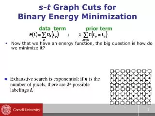
Find Labeling 5 2 1 3 4 2 1 3 5 4 Such that the sum of the assignment costs and separation costs (the energy E) is small Pixel labeling problem Given Assignment cost for giving a particular label to a particular node. Written as D. Separation cost for assigning a particular pair of labels to neighboring nodes. Written as V.
Solving pixel labeling problems • We want to minimize the energy E(f) • Problem show up constantly in vision • And in other fields as well • Bayesian justification (MRF’s)
Stereo Pixel labeling for stereo • Labels are shifts (disparities, hence depths) • At the right disparity, I1(p) I2(p+d) • Assignment cost is D(p,d) = (I1(p) – I2(p+d))2 • Neighboring pixels should be at similar depths • Except at the borders of objects!
Classical solutions • No good solutions until recently • General purpose optimization methods • Simulated annealing, or some such • Bad answers, slowly • Local methods • Each pixel chooses a label independently • Bad answers, fast
Graph cuts Slow Right answers Slow (annealing) Fast (correlation) Fast How fast do you want the wrong answer?
What do graph cuts provide? • For less interesting V, polynomial algorithm for global minimum! • For a particularly interesting V, approximation algorithm • Proof of NP hardness • For many choices of V, algorithms that find a strong local minimum • Very strong experimental results
Part A: Graph Cuts Everything you never wanted to know about cuts and flows (but were afraid to ask)
Max flow problem: Each edge is a “pipe” Find the largest flow F of “water” that can be sent from the “source” to the “sink” along the pipes Edge weights give the pipe’s capacity a flow F “source” “sink” T S A graph with two terminals Maximum flow problem
Min cut problem: Find the cheapest way to cut the edges so that the “source” is completely separated from the “sink” Edge weights now represent cutting “costs” a cut C “source” “sink” T S A graph with two terminals Minimum cut problem
Max Flow = Min Cut: Maximum flow saturates the edges along the minimum cut. Ford and Fulkerson, 1962 Problem reduction! Ford and Fulkerson gave first polynomial time algorithm for globally optimal solution “source” “sink” T S A graph with two terminals Max flow/Min cut theorem
Fast algorithms for min cut • Max flow problem can be solved fast • Many algorithms, we’ll sketch one • This is not at all obvious • Variants of min cut are NP-hard • Multiway cut problem • More than 2 terminals • Find lowest cost edges separating them all
“source” “sink” T S A graph with two terminals “Augmenting Path” algorithms • Find a path from S to T along non-saturated edges • Increase flow along this path until some edge saturates
“source” “sink” T S A graph with two terminals “Augmenting Path” algorithms • Find a path from S to T along non-saturated edges • Increase flow along this path until some edge saturates • Find next path… • Increase flow…
“source” “sink” T S A graph with two terminals “Augmenting Path” algorithms • Find a path from S to T along non-saturated edges • Increase flow along this path until some edge saturates Iterate until … all paths from S to T have at least one saturated edge
Implementation notes • There are many fast flow algorithms • Augmenting paths depends on ordering • Breadth first = Edmonds-Karp • Vision problems have many short paths • Subtleties needed due to directed edges • [BK ’04] gives an algorithm especially for vision problems • Software is freely available
Part B: Graph cuts in vision How you can turn vision problems into min cut problems for fun and profit (or, not)
A surprising result • Minimizing E in vision is difficult • Huge search space • Many local minima • With 2 labels, can find the global min! • [Greig, Porteus, Shehult, 1986] • Problem reduction to min cut
0 1 Construction • Exactly 1 green link is cut, for every pixel • Cuts are labelings • Two obvious encodings • If two adjacent pixels end up linked to different terminals, the black link between them must be cut • Cost of cut is energy of labeling
Smoothness term matters • V determines what the solution prefers • Consider uniform D • Comes from the MRF’s prior • Convex V over-penalizes discontinuities |d1 – d2| • Non-convex V is important T[d1 != d2], called the Potts model min(|d1 - d2|,K)
Why is the problem hard? • Minimizing the energy for the interesting choices of V is NP-hard • Problem reduction from multiway cut • Result is somewhat recent [BV&Z ’01] • Requires exponential search • Dimension = number of pixels
Convex V is easy • Graph cuts can rapidly compute the global minimum • Convex V, contiguous integer labels • [Ishikawa ’04] • Another amazing result • Not of practical interest (IMHO) • You can really see the over-smoothing
Local minima and moves • A local minimum is all we can hope for • For the important class of V • Minimum relative to a set of moves • Better than any “nearby” solution • We will compute a local minimum with respect to very powerful moves
Green-yellow swap move Red expansion move Starting point
Swap move algorithm • 1. Start with an arbitrary labeling • 2. Cycle through every label pair (,) in some order • 2.1 Find the lowest Elabeling within a single ,-swap • 2.2 Go there if this has lower E than the current labeling • 3. If E did not decrease in the cycle, we’re done. Otherwise, go to step 2
Expansion move algorithm • 1. Start with an arbitrary labeling • 2. For each label in some order • 2.1 Find the lowest E labeling within a single -expansion • 2.2 Go there if this has lower E than the current labeling • 3. If E did not decrease in the cycle, we’re done. Otherwise, go to step 2
Algorithm properties • In a cycle the energy E doesn’t increase • These are greedy methods • Convergence guaranteed in O(n) cycles • In practice, termination occurs in a few cycles • When the algorithms converge, the resulting labeling is a local minimum • Even when allowing an arbitrary swap move or expansion move
Strong local minima • A local minimum with respect to these moves is the best answer in a very large neighborhood • For example, there are O(k 2n) labelings within a single expansion move • Starting at an arbitrary labeling, you can get to the global minimum in k expansion moves • The expansion move algorithm yields a 2-approximation for Potts model V
Binary sub-problem • The input problem involves k labels, but the key sub-problem involves only 2 • Minimize Eover all O(2n) labelings within a single -expansion move from f • Each pixel peither keeps its old label fp, or acquire the new label • Classical problem reduction • To min cut problem
Part C: What energy functions can graph cuts minimize? Or, what else can we do with this?
Different D example • Birchfield-Tomasi method • Compute an intensity interval • Use this as basis for D(p,d) • Handles sampling error
Different V example Stereo Image: White rectangle moves one pixel, background is stationary
0 C D E B vq vr vp A F G 1 Cuts are binary labelings
Recent progress • Over the last 4 years several such problem reductions have been done • Graph constructions have been specialized to a particular E, and quite complex • You can’t tell by looking at E whether such a construction is possible, let alone how to do it • We now have a much more general result for energy functions of binary-valued variables • Graph cuts invariably use binary variables
Energy functions and graphs • Consider Ewhich assigns to any cut (binary labeling) the cost of that cut • Computing the min cut on G is a fast way to find the labeling that minimizes E • We will say that GrepresentsE • Every weighted graph with two terminals represents some energy function • What we really want is to go in the opposite direction!
Basic questions • For what energy functions Ecan we construct a graph Gthat represents E? • I.e., what energy functions can we efficiently minimize using graph cuts? • How can we easily construct the graph Gthat represents E? • I.e., given an arbitrary Ethat we know to be graph-representable, how do we find G?
Question #1 What class of energy functions can we efficiently minimize using graph cuts?
Functions in F3 can be written as The classes F2 and F3 • Consider functions of n binary variables • Functions in F2 can be written as
Regularity • All functions E of 1 binary variable are defined to be regular • A function E of 2 binary variables is regular if • A function E of more than 2 binary variables is regular if all its projections are regular
Regularity theorem • A graph-representable function of binary variables must be regular • In fact, minimizing an arbitrary non-regular functions in F2 is NP-hard • Reduction from independent set problem
F3 Theorem • Any regular function in F3 is graph-representable • With the regularity theorem, this completely characterizes the energy functions E that can be efficiently minimized with graph cuts • Assuming E has no terms with >3 variables
Question #2 Given: an arbitrary graph- representable E Question: How do we find G ?
Desired construction • Input: an arbitrary regular EF3 • Output: the graph that represents E
Additivity theorem • The sum of two graph-representable energy functions is itself graph-representable • Assume that the two graphs are defined on the same sets of vertices, i.e. they differ only in the edge weights • We simply add the edge weights together • If there is no edge, we can pretend there is one with weight 0
Regrouping theorem • Any regular function in F3 can be re-written as the sum of terms, where each term is regular and involves 3 or fewer variables • Combined with the additivity theorem, we need only build a graph for an arbitrary regular term involving 3 or fewer variables
Construction for F2 • Consider an arbitrary regular E in F2 • We only need to look at a single term, whose form is like D(vp) or V(vp,vq) • Example: expansion moves for stereo • We will show how the construction works for both types of terms • Each term is known to be regular!
Data terms • We need a graph construction that imposes one “penalty” if vp = 0, but another if vp = 1 • The “penalty” can be positive or negative!
Rewriting the penalty • The penalty Z = E(0) – E(1), imposed iff vp = 0, can be positive or negative • But graph has non-negative edge weights!