Reinforcement Learning Rules in Computational Neuroscience
Explore the Rescorla-Wagner rule in reinforcement learning for classical conditioning paradigms and animal behavior. Understand static and sequential action choice in a two-armed bandit problem and learn about exploration versus exploitation trade-offs using stochastic policies. Discover indirect and direct actor reinforcement learning schemes and temporal difference learning for future rewards.

Reinforcement Learning Rules in Computational Neuroscience
E N D
Presentation Transcript
Learning Rules 2 Computational Neuroscience 03 Lecture 9
Reinforcement Learning In reinforcement learning we have a stimulus s a reward r and an expected reward v. We represent the presence or absence of the stimulus by a binary variable u (apologies for confusion over labels: this follows convention in the literature) Where the weight w is established by a learning rule which minimises the mean square error between expected reward and actual reward (note similarities to ANN training) Using this terminology have the Rescorla-Wagner rule (1972): Where e is learning rate (form of stochastic gradient descent)
If e is sufficinetly small and u = 1 on all trials the rule makes w fluctuate about the equilibrium value w=<r> Using the above rule can get most of the classical conditioning paradigms (where -> indicates an association between a one or 2 stimuli and a reward (r) or the absence of a reward. In the result column the association is with an expectaion of a reward)
For instance here we can see acquisition, extinction and partial reinforcement. Can also get blocking, inhibitory conditioning and overshadowing. However, cannot get secondary conditioning due to lack of a temporal dimension and the fact that reward is delayed
But how are these estimates of expected reward used to determine an animal’s behaviour? Idea is that animal develops a policy (plan of action) aimed at maximising the reward that it gets Thus the policy is tied into its estimate of the reward If reward/punishment follows action immediately we have what’s known as static action choice If rewards are delayed until several actions are completed have sequential action choice
Static Action Choice Suppose we have bees foraging in a field of 20 blue and 20 yellow flowers Blue flowers give a reward of rb of nectar drwan from a probability distribution p(rb ) Blue flowers give a reward of ry of nectar drwan from a probability distribution p(ry ) Forgetting about spatial aspects of foraging we assume at each timestep the beeis faced with ablue or yellow flower and must choose between them: task known as a stochastic two-armed bandit problem
Bee follows a stochastic policy parameterised by 2 which means it chooses flowers with probability P(b) and P(y) where convenient to choose: Here mb and my the action values parameterise the probabilities and are updated using a learning process based on expected and received rewards If there are multiple actions, use a vector of action values m Note P(b) = 1 - P(y) Also, note that both are sigmoidal functions of b(mb-my). Thus the sensitivity of probabilities to the action values is governed by b.
Exploration vs Exploitation If b is large and mb>my P(b) is almost one => deterministic sampling: Exploitation Low b implies more random sampling (b=0 => P(b)=P(y)=0.5). Exploration Clearly need a trade-off between exploration and exploitation as we must keep sampling all flowers to get a good estimate of reward but this comes at a cost of not getting optimal nectar
Indirect Actor First learning scheme is to learn average nectar volumes for each type of flower ie set mb= <rb> and my= <ry> Indirect Actor scheme as policy is mediated indirectly by the total expected nectar volumes received Using Rescorla-Wagner rule we saw that w stabilises at <r>. Therefore we use this reinforcement learning rule (with u =1 always) to update the m’s via
Results for models bees using the indirect actor scheme. <ry>=2 and <rb>=1 for 1st 100 visits. Then reward values swapped (<ry>=1 and <rb>=2) for 2nd 100. A shows mb and my. B-D shows cumulative visists to each type of flower. B b = 1 C+D b = 50 From results we can see that with a low b value (b =1) (fig B), learning is slow but change to optimal flower colour is reliable For a high b value (b =50), sometimes get optimal behaviour (C) but sometimes get suboptimal (D) However, such a scheme would have trouble if eg ry=2 always while rb=6 1/3 of the time and rb=0 2/3 of time
Direct actor schemes try to maximise expected reward directly ie use <r>= P(b) <rb> + P(y) <ry> And maximise over time using stochastic gradient ascent Direct Actor Same task as previous slide. One run has quite good results (A, B) while other has bad results (C,D) Results for this rule are quite variable and behaviour after reward change can be poor. However direct actor can be useful to see how action choice can be separated from action evaluation
Temporal difference learning Imagine we have a stimulus presented at t=5 but the reward not given till t=10. To be able to learn based on future rewards, need to add a temporal dimension to Rescorla-Wagner Use a discrete time variable t where 0<= t <= T and stimulus u(t), prediction v(t) and reward r(t) are all functions of t Here now v(t) is interpreted as the expected future reward from time t to T as this provides a better match to empirical data ie And the learning rule becomes: where
How does this work? Imagine we have a trial 10 timesteps long with a single stimulus at t=5 and a reward of 0.5 at t=10. For the case of a single stimulus have: So: v(0) = w(0)u(0) v(1) = w(0)u(1) + w(1)u(0) v(2) = w(0)u(2) + w(1)u(1) + w(2)u(0) v(3) = w(0)u(3) + w(1)u(2) + w(2)u(1) etc … So, since u(t)=0 except for t = 5 where u=1, we have v(t)=0 for t<5 and: v(5)= w(0)u(5)= w(0), v(6)= w(1)u(5) = w(1), v(7)=w(2), v(8)= w(3), v(9)=w(4), v(10)= w(5), Ie v(t) = w(t-5)
At the start (Trial 0) all w =0. Therefore all v=0. Remembering that: we therefore get: d(t) = 0 for t < 10 and d(10) = 0.5 Also, as with calculating the v’s, since u(t)=0 for all t not 5 and u(5) =1 when calculating increase in w need: t – t = 5 ie t = t + 5 Therfore setting e = 0.1 get
Trial 1: d(t) = 0 for t < 10 and d(10) = 0.5 w’s unless t+5=10 ie t=5 d = 0 so w(5) = 0 + 0.1 d(10) = 0.05 all other w’s zero as other d’s are zero v’s unless t-5 = 5 w = 0 so all v zero apart from v(10) = 0.05 d’s d(10) = r(10) + v(11) – v(10) = 0.5 + 0 – 0.05 = 0.45 d(9) = r(9) + v(10) – v(9) = 0 + 0.05 – 0 = 0.05 rest are 0
Trial 2: d(10) = 0.45, d(9) = 0.05 w’s Now need either t+5=10 (t=5) or t+5=9 (t=4) so: w(5) -> w(5) + 0.1 d(10) = 0.05 + 0.1x0.45 = 0.095 w(4) -> w(4) + 0.1 d(9) = 0 + 0.1x0.05 = 0.005. other w’s = zero v’s unless t-5 = 5 or t-5 =4 w = 0 so v(10)=w(5)=0.095, v(9)=w(4)=0.005 d’s d(10) = r(10) + v(11) – v(10) = 0.5 + 0 – 0.95 = 0.405 d(9) = r(9) + v(10) – v(9) = 0 + 0.095 – 0.005 = 0.09 d(8) = r(8) + v(9) – v(8) = 0 + 0.005 – 0 = 0.005 others zero
Trial 100 w’s: w(6) and more = 0 since then add on d(11) = 0. w(5) and lower keep increasing until they hit 0.5. Why do they stop then? If w(5)=0.5 then v(10)=0.5, so d(10) = r(10) + v(11) –v(10) = 0.5 + 0 – 0.5 = 0 ie no change to w(5) And if w(4) =0.5, v(10)=v(9)=0.5 d(9)=r(9)+v(10)–v(9)=0.5–0.5 = 0 Therefore no change to w(4) and if w(3) = 0.5, d(8)=0 , so no change etc
Trial 100 v’s: So since w(0)-w(5)=0.5, rest zero v(10)-v(5) = 0.5, rest zero And d’s: d(10) = r(10) + v(11) –v(10) = 0.5 + 0 – 0.5 = 0 d(9) = r(9) + v(10) –v(9) = 0+0.5 – 0.5 = 0 and same for d(8), d(7), d(6), d(5) until we get to d(4) . Here v(5) = 0.5 but v(4)=0 so: d(4)=r(4)+v(5)–v(4)=0+0.5–0=0.5 But for d(3), v(4)=v(3)=0 so d(3)=r(3)+v(4)–v(3)=0+0–0=0 And the same for d(2), d(1), d(0)
Can see a similar effect here (stimulus at t=100, reward at t=200)
Sequential Action Choice Temporal difference (TD) learning is needed in cases where the reward does not follow immediately after the action. Consider the maze task below: While we could use static action choice to get actions at B and C, we don’t know what reward we get for turning left at A Use policy iteration. Have a stochastic policy which is maintained and updated and determines actions at each point
Actor-Critic Learning Have 2 elements: A critic which uses TD learning to estimate the future reward from A, B and C if current policy followed An actor which maintains and improves the policy based on the values from the critic Effectively, rat still uses static action choice at A but using the expectation of the future reaward from the critic
Eg rat in a maze. Initially rat has no preference for left or right ie m=0 so probability of going either way is 0.5.Thus: v(B) = 0.5(0 + 5) = 2.5, v(C) = 0.5(0 + 2) = 1, v(A) = 0.5(v(B) + v(C)) = 1.75 These are future rewards expected if rat explores maze using random choices. These can be learnt via TD learning. Here if rat chooses action a at location u and ends up at u’ have: where
Get results as above. Dashed lines are correct expected rewards. Learning rate of 0.5 (fast but noisy). Thin solid lines are actual values, thick lines are running averages of the weight values. Weights converge to the true values of the rewards This process is known as polcy evaluation
Now use policy improvement where the worth to rat if it takes action a at u and moves to u’ is sum of reward received and rewards expected to follow ie ra(u) + v(u’) Policy improvement uses the difference between this reward and the total expected reward v(u) This value is then used to update the policy
Eg suppose we start from location A. Using the true values of the locations evaluated earlier get For a left turn For a right turn This means that the policy is adapted to increase the probability of tuning left as learning rule increases probability for d > 0 and decreases probability for d < 0
Strictly, policy should be evaluated fully before policy is improved and more straightforward to improve policy fully before policy re-evaluated However, a convenient (but not provably correct alternative) is to interleave partial policy evaluation and policy improvement steps This is known as the actor-critic algorithm and generates the results above
Actor-Critic Generalisations Actor critic rule can be generalised in a number of ways eg 1. Discounting rewards: more recent rewards/punishments have more effect. In calculating expected future reward, multiply the reward by gt where t is the number of time-steps until the reward is received and 0<= g <= 1. The smaller g the stronger the effect of discounting. This can be implemented simply by changing d to be:
2. Multiple sensory information at a point a. Eg as well as having a stimulus at a there is also a food scent. Instead of having u represented by a binary variable we therefore have a vector u which parameterises the sensory input (eg stimulus and scent would be a 2 element vector. Vectors for maze would be u(A) = (1, 0, 0), u(B) = (0, 1, 0), u(C) = (0, 0, 1) where sensory info is ‘at A’ ‘at B’ and ‘at C’). Now v(u) = w.u so need w to be a vector of same length. Thus: w->w +edu(a) and need M as a matrix of probabilities so that m = M.u
3. Learning usually based on difference between immediate reward and one from the next timestep. Instead can base learning rules on the sum of next 2, 3 or more immediate rewards and the estimate of future rewards on more temporally distant timesteps. Using l to weight our future estimates this can be achieved using eg the recursive rule: Basically takes into account some measure of past activity. l = 0: new u = standard u and no notice taken of past. l = 1: no notice taken of present

