Download
1 / 11
110 likes | 128 Vues
Understanding the FAUST algorithm for detecting outliers in big data, including FAUST One-Class Spherical and Linear classifiers. Strategies for fast, analytic, unsupervised, and supervised outlier identification using FAUST technology.

E N D
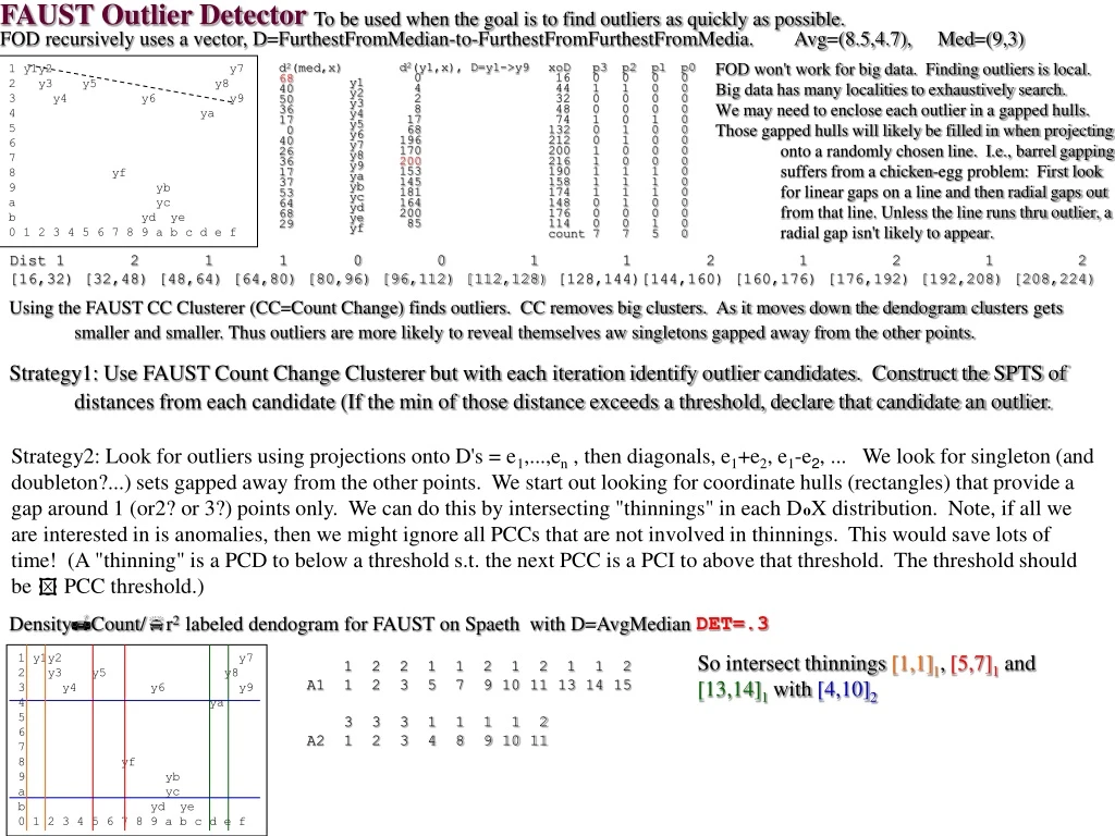
DensityCount/r2 labeled dendogram for FAUST on Spaeth with D=AvgMedian DET=.3 1 y1y2 y7 2 y3 y5 y8 3 y4 y6 y9 4 ya 5 6 7 8 yf 9 yb a yc b yd ye 0 1 2 3 4 5 6 7 8 9 a b c d e f So intersect thinnings [1,1]1, [5,7]1 and [13,14]1 with [4,10]2 1 2 2 1 1 2 1 2 1 1 2 A1 1 2 3 5 7 9 10 11 13 14 15 3 3 3 1 1 1 1 2 A2 1 2 3 4 8 9 10 11 Dist 1 2 1 1 0 0 1 [16,32) [32,48) [48,64) [64,80) [80,96) [96,112) [112,128) 1 2 1 2 1 2 [128,144)[144,160) [160,176) [176,192) [192,208) [208,224) FAUST Outlier Detector To be used when the goal is to find outliers as quickly as possible. FOD recursively uses a vector, D=FurthestFromMedian-to-FurthestFromFurthestFromMedia. Avg=(8.5,4.7), Med=(9,3) 1 y1y2 y7 2 y3 y5 y8 3 y4 y6 y9 4 ya 5 6 7 8 yf 9 yb a yc b yd ye 0 1 2 3 4 5 6 7 8 9 a b c d e f FOD won't work for big data. Finding outliers is local. Big data has many localities to exhaustively search. We may need to enclose each outlier in a gapped hulls. Those gapped hulls will likely be filled in when projecting onto a randomly chosen line. I.e., barrel gapping suffers from a chicken-egg problem: First look for linear gaps on a line and then radial gaps out from that line. Unless the line runs thru outlier, a radial gap isn't likely to appear. d2(y1,x), D=y1->y9 0 4 2 8 17 68 196 170 200 153 145 181 164 200 85 xoD p3 p2 p1 p0 16 0 0 0 0 44 1 1 0 0 32 0 0 0 0 48 0 0 0 0 74 1 0 1 0 132 0 1 0 0 212 0 1 0 0 200 1 0 0 0 216 1 0 0 0 190 1 1 1 0 158 1 1 1 0 174 1 1 1 0 148 0 1 0 0 176 0 0 0 0 114 0 0 1 0 count 7 7 5 0 d2(med,x) 68 40 50 36 17 0 40 26 36 17 37 53 64 68 29 y1 y2 y3 y4 y5 y6 y7 y8 y9 ya yb yc yd ye yf Using the FAUST CC Clusterer (CC=Count Change) finds outliers. CC removes big clusters. As it moves down the dendogram clusters gets smaller and smaller. Thus outliers are more likely to reveal themselves aw singletons gapped away from the other points. Strategy1: Use FAUST Count Change Clusterer but with each iteration identify outlier candidates. Construct the SPTS of distances from each candidate (If the min of those distance exceeds a threshold, declare that candidate an outlier. Strategy2: Look for outliers using projections onto D's = e1,...,en , then diagonals, e1+e2, e1-e2, ... We look for singleton (and doubleton?...) sets gapped away from the other points. We start out looking for coordinate hulls (rectangles) that provide a gap around 1 (or2? or 3?) points only. We can do this by intersecting "thinnings" in each DoX distribution. Note, if all we are interested in is anomalies, then we might ignore all PCCs that are not involved in thinnings. This would save lots of time! (A "thinning" is a PCD to below a threshold s.t. the next PCC is a PCI to above that threshold. The threshold should be PCC threshold.)
FAUST Hull ClassifiersFast, Analytic, Unsupervised and Supervised Technology C = class, X = unclassified samples, r = a chosen minimum gap threshold. FAUST One-Class Spherical (OCS) FAUST Multi-Class Spherical (MCS) Classify x as class C iff the count of cCk s.t.(c-x)o(c-x) r2 is max Classify x as class C iff there exists cC such that (c-x)o(c-x) r2 a a a a a a a a aa a a a a aa a c c c c c c c c cc c c c c cc c b b b b b b b b bb b b b b bb b D=e1+e2+e3 D=e1-e3 e3 e2 D=e1+e3 e1 mxBoD12 mxCoD12 mnC1 mxC1 mnA1 mnB1 mxB1 mxA1 mnCoD12 mxAoD12 mnBoD12 mnAoD12 FAUST One-Class Linear (OCL)Construct a hull, H, around C. x is class C iff xH. For a series of vectors, D, let loDmnCoD (or the 1st PCI); hiDmxCoD (or the last PCD). Classify xC iff loD Dox hiD D. E.g., let the D-series be the diagonals e1, e2, ...en, e1+e2, e1-e2, e1+e3, e1-e3, ...,e1-e2-...-en? (add more Ds until diamH-diamC < ε? FAUST Multi-Class Linear (MCL)Construct a hull, Hk, about Ck k as above. Then x isa Ck iff k, xHk. (allows for a "none of the classes" when xHk, k.) The Hks can be constructed in parallel: Convex hull Our hull, H c c c c c c c c cc c c c c cc c D12=e1-e2 line 3D example of HULL1 e1 line 1-class classification Reference : http://homepage.tudelft.nl/n9d04/thesis.pdf#appendix*.7
FAUST OCS One Class Spherical classifier on the Spaeth dataset as a "lazy" classifier So yf is not in C since it is spherically gapped away from C by r=3 units. How expensive is the algorithm? For each x 1. Compute SPTS, (C-x)o(C-x) 2. Compute mask pTree (C-x)o(C-x)< r2 3. Count 1-bits in that mask pTree. Let the Class be {yb,yc.yd,ye}. OCS classify x=yf. Let r=3. C1 pTrees C2 pTrees C C1 13 12 11 10 C2 23 22 21 20 (c-x)o(c-x) yb 10 1 0 1 0 9 1 0 0 1 10 yc 11 1 0 1 1 10 1 0 1 0 20 yd 9 1 0 0 1 11 1 0 1 1 13 ye 11 1 0 1 1 11 1 0 1 1 25 yf 7 0 1 1 1 8 1 0 0 0 0 1 y1y2 y7 2 y3 y5 y8 3 y4 y6 y9 4 ya 5 6 7 8 yf 9 yb a yc b yd ye 0 1 2 3 4 5 6 7 8 9 a b c d e f Shortcut for 1.d,e,f by some comparison of hi bitslices of (C-x)o(C-x) with #9? (I think Yue Cui has a shortcut ???) C1 13 12 11 10 C2 23 22 21 20 yb 10 1 0 1 0 9 1 0 0 1 yc 11 1 0 1 1 10 1 0 1 0 yd 9 1 0 0 1 11 1 0 1 1 ye 11 1 0 1 1 11 1 0 1 1 x=yf 7 0 1 1 1 8 1 0 0 0 C as a PTS is: and x=yf: Shortcut for 1.a,b,c,d,e,f: (C-x)o(C-x) = CoC -2Cox +|x|2 < r2 |x|2-r2 + CoC < 2Cox #7 3 2 1 0 #8 3 2 1 0 #9 3 2 1 0 7 0 1 1 1 8 1 0 0 0 9 1 0 0 1 7 0 1 1 1 8 1 0 0 0 9 1 0 0 1 7 0 1 1 1 8 1 0 0 0 9 1 0 0 1 7 0 1 1 1 8 1 0 0 0 9 1 0 0 1 1a Compute SPTS (C-x)o(C-x): 1.f Conclude that yfC 1.b Form cosntant SPTSs 1.e Count the 1 bits = 0 1.c Construct (C-x)o(C-x) by SPTS arithmetic: (C-x)o(C-x)=(C1-#7)(C1-#7) + (C2-#8)(C2-#8) 4 3 2 1 0 10 0 1 0 1 0 20 1 0 1 0 0 13 0 1 1 0 1 25 1 1 0 0 1 0 0 0 0 1.d Construct the mask pTree (C-x)o(C-x)<#9 Precompute (1 time) SPTS CoC and PTS 2C (2C is just a re-labeling (shift left) of pTrees of C). For each new unclassified sample, x, add |x|2-r2 to CoC (adding one constant to one SPTS) compute 2Cox (n multiplications of one SPTS, 2Ci, by one constant, xi' then add the n resulting SPTSs. compare |x|2-r2 +CoC to 2Cox giving us a mask pTree. Count 1-bits in this mask pTree (shortcuts?, shortcuts?, shortcuts?) CoC pTrees CoC 7 6 5 4 3 2 1 0 181 1 0 1 1 0 1 0 1 221 1 1 0 1 1 1 0 1 202 1 1 0 0 1 0 1 0 242 1 1 1 1 0 0 1 0 2C1 pTrees 2C2 pTrees 2C1 14 13 12 11 2C2 24 23 22 21 20 1 0 1 0 18 1 0 0 1 22 1 0 1 1 20 1 0 1 0 18 1 0 0 1 22 1 0 1 1 22 1 0 1 1 22 1 0 1 1 a = |x|2-r2 = 104 CoC+a pTrees CoC+a 8 7 6 5 4 3 2 1 0 285 1 0 0 0 1 1 1 0 1 325 1 0 1 0 0 0 1 0 1 306 1 0 0 1 1 0 0 1 0 346 1 0 1 0 1 1 0 1 0 2Cox pTrees 2Cox 8 7 6 5 4 3 2 1 0 284 1 0 0 0 1 1 1 0 0 314 1 0 0 1 1 1 0 1 0 302 1 0 0 1 0 1 1 1 0 330 1 0 1 0 0 1 0 1 0 CoC+a>2Cox 0 0 0 0 Ct=0 so x not in C 1class classify unclassified sample, x=(a,9). Let r=3. CoC+a pTrees CoC+a 9 8 7 6 5 4 3 2 1 0 724 1 0 1 1 0 1 0 1 0 0 884 1 1 0 1 1 1 0 1 0 0 808 1 1 0 0 1 0 1 0 0 0 968 1 1 1 1 0 0 1 0 0 0 2Cox pTrees 2Cox 8 7 6 5 4 3 2 1 0 362 1 0 1 1 0 1 0 1 0 400 1 1 0 0 1 0 0 0 0 378 1 0 1 1 1 1 0 1 0 418 1 1 0 1 0 0 0 1 0 CoC+a>2Cox 1 1 1 1 Ct=4 so x in C
For WINE with C=class4 and outliers=class7 (Class 4 was enhanced with 3 class3's to fill out the 50) For CONCRETE, concLH with C=class(8-40) and outliers=class(43-67) The 1D model classifies 50 class1 and 43 class3 incorrectly as class1. The 1D model classifies 50 class1 and 48 class3 incorrectly as class1. For SEEDS with C=class1 and outliers=class2 For IRIS with C=Vers, outliers=Virg,FAUST 1D: SLcutpts (49,70); SWcutpts(22,32); PLcutpts(33,49); PW Ctpts(10,16) 44 vers correct. 7 virg errors The 1D model classifies 50 class1 and 15 class2 incorrectly as class1. The 1D_2D model classifies 50 class1 and 43 class3 incorrectly as class1. The 1D_2D model classifies 50 class1 and 35 class3 incorrectly as class1. Trim outliers: 20;34 30:50,51 18 The 1D_2D model classifies 50 class1 and 8 class2 incorrectly as class1. The 1D_2D_3D model classifies 50 class1 and 30 class3 incorrectly as class1. The 1D_2D_3D model classifies 50 class1 and 43 class3 incorrectly as class1. The 1D_2D_3D model classifies 50 class1 and 8 class2 incorrectly as class1. 1D_2D model classifies 50 vers (no eliminated outliers) and 3 virg in the 1class The 1D_2D_3D_4D model classifies 50 class1 and 27 class3 incorrectly as class1. The 1D_2D_3D_4D model classifies 50 class1 and 42 class3 incorrectly as class1. The 1D_2D_3D_4D model classifies 50 class1 and 8 class2 incorrectly as class1. 1D_2D_3D model classifies 50 vers (no eliminated outliers) and 3 virg in the 1class For CONCRETE, concM (class is the middle range of strengths) The 1D model classifies 50 class1 and 47 class3 incorrectly as class1. 1D_2D_3D_4D model classifies 50 vers (no eliminated outliers) and 3 virg in the 1class For SEEDS with C=class1 and outliers=class3 The 1D_2D model classifies 50 class1 and 37 class3 incorrectly as class1. The 1D model classifies 50 class1 and 30 class3 incorrectly as class1. The 1D_2D_3D model classifies 50 class1 and 30 class3 incorrectly as class1. The 1D_2D model classifies 50 class1 and 27 class3 incorrectly as class1. The 1D_2D_3D model classifies 50 class1 and 27 class3 incorrectly as class1. The 1D_2D_3D_4D model classifies 50 class1 and 26 class3 incorrectly as class1. The 1D_2D_3D_4D model classifies 50 class1 and 27 class3 incorrectly as class1. For SEEDS with C=class2 and outliers=class3 The 1D model classifies 50 class1 and 0 class3 incorrectly as class1. The 1D_2D model classifies 50 class1 and 0 class3 incorrectly as class1. The 1D_2D_3D model classifies 50 class1 and 0 class3 incorrectly as class1. The 1D_2D_3D_4D model classifies 50 class1 and 0 class3 incorrectly as class1. FAUST OCL One Class Linearclassifier applied to IRIS, SEEDS, WINE, CONCRETE datasets For series of D's = diagonals e1, e2, ...en, e1+e2, e1-e2, e1+e3, e1-e3, ...,e1-e2-...-en The 3 persistent virg errors virg24 63 27 49 18 virg27 62 28 48 18 virg28 61 30 49 18
Class1=C1={y1,y2.y3,y4. FAUST MCL C e1 13 12 11 10 e2 23 22 21 20 y1 1 0 0 0 1 1 0 0 0 1 y2 3 0 0 1 1 1 0 0 0 1 y3 2 0 0 1 0 2 0 0 1 0 y4 3 0 0 1 1 3 0 0 1 1 y7 15 1 1 1 1 1 0 0 0 1 y8 14 1 1 1 0 2 0 0 1 0 y9 15 1 1 1 1 3 0 0 1 1 yb 10 1 0 1 0 9 1 0 0 1 yc 11 1 0 1 1 10 1 0 1 0 yd 9 1 0 0 1 11 1 0 1 1 ye 11 1 0 1 1 11 1 0 1 1 mn1 1 mx1 3 mn2 1 mx2 3 mn1+2 2 mx1+2 6 mn1-2 0 mx1-2 2 mn1 14 mx1 15 mn2 1 mx2 3 mn1+2 16 mx1+2 18 mn1-2 12 mx1-2 14 mn1 9 mx1 11 mn2 9 mx2 11 mn1+2 20 mx1+2 22 mn1-2 -1 mx1-2 1 Class2=C2={y7,y8.y9}. xCk iff lok,D Dox hik,D D. Class3=C3={yb,yc.yd,ye} 1 y1y2y7 2 y3y5 y8 y 3 y4 y6 y9 4 ya 5 6 7 8 yf 9 yb ax yc b yd ye 0 1 2 3 4 5 6 7 8 9 a b c d e f Shortcuts for MCL? Pre-compute all diagonal minimums and maximums; e1, e2, e1+e2, e1-e2. Then in fact, there is no pTree processing left to do (just straight forward number comparisons). xf 7 On basis of e1 it is "none-or-the-above" 9,a 9 -1 19 10 It is in class3 (red) only ya 13 On the basis of e1 it is "none-or-the-above" Versicolor 1D min 49 20 33 10 max 70 34 51 18 n1 n2 n3 n4 x1 x2 x3 x4 y5 5 2 On the basis of e1 it is "none-or-the-above" f,2 15 13 17 2 It is in class2 (green) only 1D MCL Hversicolor has 7 virginica! Versicolor 2D min 70 82 59 55 59 43 24 9 38 -24 7 23 max 102 118 84 80 84 67 40 23 56 -7 18 35 n12 n13 n14 n23 n24 n34 n1-2 n1-3 n1-4 n2-3 n2-4 n3-4 x12 x13 x14 x23 x24 x34 x1-2 x1-3 x1-4 x2-3 x2-4 x3-4 1D_2D MCL Hversicolor has 3 virginica! 1D_2D_3D MCL Hversicolor has 3 virginica! Versicolor 3D min 105 80 92 65 35 58 -21 60 35 max 149 116 134 98 55 88 -2 88 55 n123 n124 n134 n234 n12-3 n1-23 n1-2-3 n12-4 n1-24 x123 x124 x134 x234 x12-3 x1-23 x1-2-3 x12-4 x1-24 9 72 24 -7 45 -9 -40 28 103 37 12 65 6 -19 n1-2-4 n13-4 n1-34 n1-3-4 n23-4 n2-34 n2-3-4 x1-2-4 x13-4 x1-34 x1-3-4 x23-4 x2-34 x2-3-4 Versicolor 4D min 115 95 45 68 20 48 -6 -39 max 164 135 69 104 41 74 10 -12 n1234 n123-4 n12-34 n1-234 n12-3-4 n1-23-4 n1-2-34 n1-2-3-4 x1234 x123-4 x12-34 x1-234 x12-3-4 x1-23-4 x1-2-34 x1-2-3-4 1D_2D_3D_4D MCL Hversicolor has 3 virginica (24,27,28) 1D_2D_3D_4D MCL Hvirginica has 20 versicolor errors!! Look at removing outliers (gapped>=3) from Hullvirginica 23 Ct gp 48 1 22 70 1 2 72 1 3 75 2 1 ''' 96 1 1 97 1 5 102 1 3 105 1 e1 Ct gp 49 1 7 56 1 1 ... 77 4 2 79 1 e2 Ct gp 22 1 3 25 4 1 ... 36 1 2 38 2 e3 Ct gp 18 1 27 45 1 3 ... 67 2 2 69 1 e4 Ct gp 14 1 1 24 3 1 25 3 12 Ct gp 74 1 8 82 2 2 ... 117 1 13 Ct gp 78 1 16 94 1 10 104 ... 146 14 Ct gp 66 1 9 75 2 1 ... 102 1 24 Ct gp no outliers 34 Ct gp 36 1 26 62 1 3 65 1 1 ... 89 1 3 92 1 Hvirginica 12 versic Hvirginica 3 versic Hvirginica 15 versic 1D MCL Hvirginica only 16 versicolors! One possibility would be to keep track of those that are outliers to their class but are not in any other class hull and put a sphere around them. Then any unclassified sample that doesn't fall in any class hull would be checked to see if it falls in any of the class outlier spheres???
Choosing a clustering from a DEL and DUL labeled Dendogram The algorithm for choosing the optimal clustering from a labeled dendogram is as follows: Let DET=.4 and DUT=½ Since a full dendogram is far bigger than the original table, we set threshold(s), We build a partial dendogram (ending a branch when threshold(s) are met) Then a slider for density would work as follows: The user set the threshold(s). We give the clustering. The user increases threshold(s). We prune the dendogram and give clustering. The user decreases threshold(s). We build each branches down further until the new threshold(s) are exceeded and give the new clustering. We might want to also display the dendogram to the user and let him select a "node=cluster" for further analysis, etc. DEL=.1 DUL=1/6 DEL=.2 DUL=1/8 DEL=.5 DUL=½ DEL=.3 DUL=½ DEL=.4 DUL=1 DEL= DUL= DEL= DUL= DEL= DUL= DEL= DUL= DEL= DUL= DEL= DUL= DEL= DUL= A B C D E F G
Y(.15) {y6,y7,y8,y9,ya}(.17) {y7,8,9,a}(.39) {y7,y8,y9,ya}(.39) {yb,yc,yd,ye,yf}(.25) {yb,yc,yd,ye}(1.01) {yb,yc,yd,ye}(1.01) {ya}() {y5}() {y4}() {y1,y2,y3,y4}(.63) {y7,y8,y9}(1.27) {y1,y2,y3}(2.54) {y6,yf}(.08) {y6,yf}(.08) {y7,y8,y9,ya,yb.yc.yd.ye}(.07) {y7,y8,y9,ya,yb.yc.yd.ye}(.07) {y1,y2,y3,y4,y5}(.37) y1,2,3,4,5(.37 {y6}() {yf}() {y6}() {yf}() {y6,y7,y8,y9,ya,yb.yc.yd.ye,yf}(.09) {y1,y2,y3,y4,y5}(.37) 123456789abcdef {yf}() {yb,yc,yd,ye}(1.01) {y6}() {y7,y8,y9,ya}(.39) APPLYING FAUST Dendogram TO SPAETH DensityCount/r2 labeled dendogram for FAUST Cluster on Spaeth with D=Avg-to-Furthest and DensityThreshold=.3 1 3 1 0 2 0 6 2 D=Avg-to-Furthest cut at 7 and 11 1 y1y2 y7 2 y3 y5 y8 3 y4 y6 y9 4 ya 5 6 7 8 yf 9 yb a yc b yd ye c d e f 0 1 2 3 4 5 6 7 8 9 a b c d e f D=Avg-to-Furth DensityThresh=.5 D=Avg-to-Furth DensityThresh=1 D-line Labeled dendogram for FAUST Cluster on Spaeth with D=furthest-to-Avg, DensityThreshold=.3 1 y1y2 y7 2 y3 y5 y8 3 y4 y6 y9 4 ya 5 6 7 8 yf 9 yb a yc b yd ye 0 1 2 3 4 5 6 7 8 9 a b c d e f DCount/r2 labeled dendogram for FAUST Clusteron Spaeth with D=cylces thru diagonals nnxx,nxxn,nnxx,nxxn..., DensThresh=.3 Y(.15) Y(.15)
applied to S, a column of numbers in bistlice format (an SpTS), will produce the DistributionTree of S DT(S) depth=h=0 15 p6' 1 1 1 1 1 0 0 0 0 0 0 0 0 0 0 5/64 [0,64) p6' 1 1 1 1 1 0 0 0 0 0 0 0 0 0 0 p6' 1 1 1 1 1 0 0 0 0 0 0 0 0 0 0 p6' 1 1 1 1 1 0 0 0 0 0 0 0 0 0 0 p6' 1 1 1 1 1 0 0 0 0 0 0 0 0 0 0 p5' 1 1 1 0 0 1 0 0 0 0 0 0 0 0 1 p5' 1 1 1 0 0 1 0 0 0 0 0 0 0 0 1 p5' 1 1 1 0 0 1 0 0 0 0 0 0 0 0 1 2/32[64,96) p4' 1 0 0 1 0 0 0 0 0 0 1 0 1 0 0 1[32,48) p5' 1 1 1 0 0 1 0 0 0 0 0 0 0 0 1 3/32[0,32) p4' 1 0 0 1 0 0 0 0 0 0 1 0 1 0 0 2[96,112) p4' 1 0 0 1 0 0 0 0 0 0 1 0 1 0 0 0[64,80) p4' 1 0 0 1 0 0 0 0 0 0 1 0 1 0 0 1/16[0,16) p5' 1 1 1 0 0 1 0 0 0 0 0 0 0 0 1 p4' 1 0 0 1 0 0 0 0 0 0 1 0 1 0 0 p5' 1 1 1 0 0 1 0 0 0 0 0 0 0 0 1 p4' 1 0 0 1 0 0 0 0 0 0 1 0 1 0 0 p5' 1 1 1 0 0 1 0 0 0 0 0 0 0 0 1 p6' 1 1 1 1 1 0 0 0 0 0 0 0 0 0 0 p4' 1 0 0 1 0 0 0 0 0 0 1 0 1 0 0 p6' 1 1 1 1 1 0 0 0 0 0 0 0 0 0 0 p4' 1 0 0 1 0 0 0 0 0 0 1 0 1 0 0 p5' 1 1 1 0 0 1 0 0 0 0 0 0 0 0 1 p6' 1 1 1 1 1 0 0 0 0 0 0 0 0 0 0 p4 0 1 1 0 1 1 1 1 1 1 0 1 0 1 1 6[112,128) p4 0 1 1 0 1 1 1 1 1 1 0 1 0 1 1 1[48,64) p3' 0 0 1 1 1 1 1 1 0 1 0 0 0 0 1 1[16,24) p4 0 1 1 0 1 1 1 1 1 1 0 1 0 1 1 2/16[16,32) p4 0 1 1 0 1 1 1 1 1 1 0 1 0 1 1 2[80,96) p4 0 1 1 0 1 1 1 1 1 1 0 1 0 1 1 p4 0 1 1 0 1 1 1 1 1 1 0 1 0 1 1 p4 0 1 1 0 1 1 1 1 1 1 0 1 0 1 1 p4 0 1 1 0 1 1 1 1 1 1 0 1 0 1 1 p5 0 0 0 1 1 0 1 1 1 1 1 1 1 1 0 p5 0 0 0 1 1 0 1 1 1 1 1 1 1 1 0 2/32[32,64) p5 0 0 0 1 1 0 1 1 1 1 1 1 1 1 0 p5 0 0 0 1 1 0 1 1 1 1 1 1 1 1 0 ¼[96,128) p5 0 0 0 1 1 0 1 1 1 1 1 1 1 1 0 p5 0 0 0 1 1 0 1 1 1 1 1 1 1 1 0 p5 0 0 0 1 1 0 1 1 1 1 1 1 1 1 0 p5 0 0 0 1 1 0 1 1 1 1 1 1 1 1 0 p3' 0 0 1 1 1 1 1 1 0 1 0 0 0 0 1 1[48,56) p3 1 1 0 0 0 0 0 0 1 0 1 1 1 1 0 1[24,32) p3 1 1 0 0 0 0 0 0 1 0 1 1 1 1 0 0[56,64) p3' 0 0 1 1 1 1 1 1 0 1 0 0 0 0 1 0[0,8) p3' 0 0 1 1 1 1 1 1 0 1 0 0 0 0 1 1[32,40) p3 1 1 0 0 0 0 0 0 1 0 1 1 1 1 0 1[8,16) p3 1 1 0 0 0 0 0 0 1 0 1 1 1 1 0 0[40,48) p6 0 0 0 0 0 1 1 1 1 1 1 1 1 1 1 10/64 [64,128) p6 0 0 0 0 0 1 1 1 1 1 1 1 1 1 1 p3' 0 0 1 1 1 1 1 1 0 1 0 0 0 0 1 2[80,88) p3' 0 0 1 1 1 1 1 1 0 1 0 0 0 0 1 3[112,120) p6 0 0 0 0 0 1 1 1 1 1 1 1 1 1 1 p6 0 0 0 0 0 1 1 1 1 1 1 1 1 1 1 p6 0 0 0 0 0 1 1 1 1 1 1 1 1 1 1 p6 0 0 0 0 0 1 1 1 1 1 1 1 1 1 1 p6 0 0 0 0 0 1 1 1 1 1 1 1 1 1 1 p6 0 0 0 0 0 1 1 1 1 1 1 1 1 1 1 p3 1 1 0 0 0 0 0 0 1 0 1 1 1 1 0 0[88,96) p3 1 1 0 0 0 0 0 0 1 0 1 1 1 1 0 3[120,128) p3' 0 0 1 1 1 1 1 1 0 1 0 0 0 0 1 p3' 0 0 1 1 1 1 1 1 0 1 0 0 0 0 1 0[96,104) p3 1 1 0 0 0 0 0 0 1 0 1 1 1 1 0 p3 1 1 0 0 0 0 0 0 1 0 1 1 1 1 0 2[194,112) UDR Univariate Distribution Revealer (on Spaeth:) 5 10 depth=h=1 node2,3 [96.128) yofM 11 27 23 34 53 80 118 114 125 114 110 121 109 125 83 p6 0 0 0 0 0 1 1 1 1 1 1 1 1 1 1 p5 0 0 0 1 1 0 1 1 1 1 1 1 1 1 0 p4 0 1 1 0 1 1 1 1 1 1 0 1 0 1 1 p3 1 1 0 0 0 0 0 0 1 0 1 1 1 1 0 p2 0 0 1 0 1 0 1 0 1 0 1 0 1 1 0 p1 1 1 1 1 0 0 1 1 0 1 1 0 0 0 1 p0 1 1 1 0 1 0 0 0 1 0 0 1 1 1 1 p6' 1 1 1 1 1 0 0 0 0 0 0 0 0 0 0 p5' 1 1 1 0 0 1 0 0 0 0 0 0 0 0 1 p4' 1 0 0 1 0 0 0 0 0 0 1 0 1 0 0 p3' 0 0 1 1 1 1 1 1 0 1 0 0 0 0 1 p2' 1 1 0 1 0 1 0 1 0 1 0 1 0 0 1 p1' 0 0 0 0 1 1 0 0 1 0 0 1 1 1 0 p0' 0 0 0 1 0 1 1 1 0 1 1 0 0 0 0 Y y1 y2 y1 1 1 y2 3 1 y3 2 2 y4 3 3 y5 6 2 y6 9 3 y7 15 1 y8 14 2 y9 15 3 ya 13 4 pb 10 9 yc 11 10 yd 9 11 ye 11 11 yf 7 8 3 2 2 8 f= 1 2 1 1 0 2 2 6 0 1 1 1 1 0 1 000 2 0 0 2 3 3 depthDT(S)b≡BitWidth(S) h=depth of a node k=node offset Nodeh,k has a ptr to pTree{xS | F(x)[k2b-h+1, (k+1)2b-h+1)} and its 1count Pre-compute and enter into the ToC, all DT(Yk) plus those for selected Linear Functionals (e.g., d=main diagonals, ModeVector . Suggestion: In our pTree-base, every pTree (basic, mask,...) should be referenced in ToC( pTree, pTreeLocationPointer, pTreeOneCount ).and these OneCts should be repeated everywhere (e.g., in every DT). The reason is that these OneCts help us in selecting the pertinent pTrees to access - and in fact are often all we need to know about the pTree to get the answers we are after.).
no carry from zero bit P1+2,1 = (P1,1 XOR P2,1) AND (NOT(P1,0&P2,0)) ... Is there a more efficient way to get the X1+X2 distribution using this route? Md? We don't need the SPTS for X1+X2 and it's expensive to create it just to get its distribution. UDR: Can we create distributionX1+2 etc. using only X1 and X2 basic ptrees (concurrently with the creation of distributionsX1, distributionX2)? An example: P2,1 0 0 1 0 P1+2,1 0 0 1 1 P1,1 1 0 0 1 X2 1 0 3 1 P2,0 1 0 1 1 X1+2 4 1 3 3 P1+2,0 0 1 1 1 X1 3 1 0 2 P1,0 1 1 0 0 P1+2,2 1 0 0 0 Let D=D1,2 e1+e2 Then DoX = 21P1,1+20P1,0 + 21P2,1+20P2,0 = 21(P1,1+P2,1) + 20(P1,0+P2,0) so we can make the 2 SPTS additions (the ones in parenthesis), shift the first left by 1 and add it to the second. But can we go directly to the UDR construction? P1+2,0 = P1,0 XOR P2,0 Md: This seems like it would give us a tremendous advantage over the "horizontal datamining boys and girls" because even though they could concurrently create all diagonal distributions, X1, X2, X1+2, X1-2, ... in one pass down the table, we would be able to do it with concurrent programs which make one pass across the SPTSs for X1 and X2.
Let's review Data Analytics Technology, Supervised and Supervised. (from Data Mining, Han, Kamber 2nd ed) I think it ia good idea to review at this point. What is the industry understanding of classification, clustering and anomaly detection. (From Han and Kamber pgs., 24-27) Classifiers(supervised analytics) construct a model that describes and distinguishes data classes or concepts, for the purpose of being able to use the model to [quickly] predict the class of objects whose class label is unknown. The derived model is based on the analysis of a set of training data (i.e., data objects whose class label is known - usually a table with a class-label column or attribute). Classification is often called "prediction" if the class labels are numbers. Classification may need to be preceded by relevance analysis to identify and eliminate attributes that do not seem to contribute much information as to class. Clusterers(unsupervised analytics) analyze data objects without consulting a known class label (ususally none are present). Clustering can be used to generate class labels in a training set that doesn't have them (create a training set) Objects are clustered (grouped) by maximizing the intra-class similarity and minimizing the inter-class similarity. Clustering can facilitate taxonomy formation, i.e., organizing objects into a hierarchy of classes that group similar events together (using a dendogram?). Anomaly Detectors(outlier detection analytics) identify objects that don't comply with the behavior of the data model Most data mining methods discard outliers as noise or exceptions. However. in some applications, such as fraud detection, the rare events can be the more interesting. Outliers may be detected using statistical tests that assume a distribution or probability model for the data, using distance measures, or deviation-based methods which identify objects by examining differences in their main characteristics. "One person's noise may be another person's signal". So outlier mining is a analytic in its own right. Outlier mining can mean: 1. Given a set of n objects and k, find the top k objects in terms of dissimilarity from the rest of the objects. 2. Given a Classification Training Set, identify objects within each class that are outliers within that class (they are correctly classified but they are noticeably dissimilar from the other objects in the class. We may find outliers for an entire set of objects (those object that don't fit into a cluster or class) and then find objects within a cluster or class that are noticeably dissimilar to the other objects in that class. I.e., find set outliers, then class outliers. 3. Given a set of objects, determine "fuzzy" clusters, i.e., assign a degree of membership for each object in each cluster. In a way, a dendogram does that. There are Statistics-based, Distance-based, Density-based and Deviation-based outlier detectors (using a dissimilarity measure, reduce the overall dissimilarity of the object set by removing "deviation outliers".).
Mohammad's results 2014_02_15: Experimental Result of Addition: Data size: 1 billion, 2 billion, 3 billion, 4 billion. Number of columns: 2 Bit width of the values: 4 bit, 8 bit, 12 bit and 16 bit . Vertical axis is time measured in millisecond. Horizontal axis is number of bit positions.