Download
1 / 79
790 likes | 877 Vues
Explore a systematic approach for Laplace problems with circular boundaries using degenerate kernels. Includes mathematical formulation, adaptive observer system, and numerical examples. Presented at BEM course on May 13, 2008.

E N D
Null-field approach for Laplace problems with circular boundaries using degenerate kernels 沈文成 陳正宗 時間:13:20 ~ 14:00 地點:河工二館 307室 BEM course May 13, 2008 (typicalBVP-L.ppt)
Outlines • Motivation and literature review • Mathematical formulation • Expansions of fundamental solution and boundary density • Adaptive observer system • Vector decomposition technique • Linear algebraic equation • Numerical examples • Degenerate scale • Conclusions
Outlines • Motivation and literature review • Mathematical formulation • Expansions of fundamental solution and boundary density • Adaptive observer system • Vector decomposition technique • Linear algebraic equation • Numerical examples • Degenerate scale • Conclusions
Motivation and literature review BEM/BIEM Improper integral Singular and hypersingular Regular Fictitious BEM Bump contour Limit process Fictitious boundary Null-field approach CPV and HPV Collocation point Ill-posed
Present approach Degenerate kernel Fundamental solution No principal value CPV and HPV Advantages of degenerate kernel 1. No principal value 2. Well-posed
Engineering problem with arbitrary geometries Straight boundary Degenerate boundary (Chebyshev polynomial) (Legendre polynomial) Circular boundary (Fourier series) (Mathieu function) Elliptic boundary
Motivation and literature review Analytical methods for solving Laplace problems with circular holes Special solution Bipolar coordinate Conformal mapping Chen and Weng, 2001, “Torsion of a circular compound bar with imperfect interface”, ASME Journal of Applied Mechanics Honein, Honein and Hermann, 1992, “On two circular inclusions in harmonic problem”, Quarterly of Applied Mathematics Lebedev, Skalskaya and Uyand, 1979, “Work problem in applied mathematics”, Dover Publications Limited to doubly connected domain
Fourier series approximation • Ling (1943) - torsion of a circular tube • Caulk et al. (1983) - steady heat conduction with circular holes • Bird and Steele (1992) - harmonic and biharmonic problems with circular holes • Mogilevskaya et al. (2002) - elasticity problems with circular boundaries
Contribution and goal • However, they didn’t employ the null-field integral equationand degenerate kernels to fully capture the circular boundary, although they all employed Fourier series expansion. • To develop a systematic approach for solving Laplace problems with multiple holes is our goal.
Outlines • Motivation and literature review • Mathematical formulation • Expansions of fundamental solution and boundary density • Adaptive observer system • Vector decomposition technique • Linear algebraic equation • Numerical examples • Degenerate scale • Conclusions
Boundary integral equation and null-field integral equation Interior case Exterior case Null-field integral equation
Outlines • Motivation and literature review • Mathematical formulation • Expansions of fundamental solution and boundary density • Adaptive observer system • Vector decomposition technique • Linear algebraic equation • Numerical examples • Degenerate scale • Conclusions
Expansions of fundamental solution and boundary density • Degenerate kernel - fundamental solution • Fourier series expansions - boundary density
Separable form of fundamental solution (1D) Separable property continuous discontinuous
Boundary density discretization Fourier series Ex . constant element Present method Conventional BEM
Outlines • Motivation and literature review • Mathematical formulation • Expansions of fundamental solution and boundary density • Adaptive observer system • Vector decomposition technique • Linear algebraic equation • Numerical examples • Degenerate scale • Conclusions
collocation point Adaptive observer system
Outlines • Motivation and literature review • Mathematical formulation • Expansions of fundamental solution and boundary density • Adaptive observer system • Vector decomposition technique • Linear algebraic equation • Numerical examples • Degenerate scale • Conclusions
Vector decomposition technique for potential gradient True normal direction Non-concentric case: Special case (concentric case) :
Outlines • Motivation and literature review • Mathematical formulation • Expansions of fundamental solution and boundary density • Adaptive observer system • Vector decomposition technique • Linear algebraic equation • Numerical examples • Degenerate scale • Conclusions
Linear algebraic equation where Index of collocation circle Index of routing circle Column vector of Fourier coefficients (Nth routing circle)
Explicit form of each submatrix [Upk] and vector {tk} Truncated terms of Fourier series Number of collocation points Fourier coefficients
Flowchart of present method Potential gradient Vector decomposition Degenerate kernel Fourier series Adaptive observer system Potential of domain point Collocation point and matching B.C. Analytical Fourier coefficients Linear algebraic equation Numerical
Outlines • Motivation and literature review • Mathematical formulation • Expansions of fundamental solution and boundary density • Adaptive observer system • Vector decomposition technique • Linear algebraic equation • Numerical examples • Degenerate scale • Conclusions
Numerical examples • Steady state heat conduction problems • Electrostatic potential of wires • Flow of an ideal fluid pass cylinders • A circular bar under torque • An infinite medium under antiplane shear • Half-plane problems
Numerical examples • Steady state heat conduction problems • Electrostatic potential of wires • Flow of an ideal fluid pass cylinders • A circular bar under torque • An infinite medium under antiplane shear • Half-plane problems
Steady state heat conduction problems Case 1 Case 2
Steady state heat conduction problems Case 3 Case 4
Case 1: Isothermal line Exact solution (Carrier and Pearson) FEM-ABAQUS (1854 elements) Present method (M=10) BEM-BEPO2D (N=21)
Convergence test - Parseval’s sum for Fourier coefficients Parseval’s sum
Case 2: Isothermal line Present method (M=10) Caulk’s data (1983) IMA Journal of Applied Mathematics FEM-ABAQUS (6502 elements)
Case 3: Isothermal line Present method (M=10) Caulk’s data (1983) IMA Journal of Applied Mathematics FEM-ABAQUS (8050 elements)
Case 4: Isothermal line Present method (M=10) Caulk’s data (1983) IMA Journal of Applied Mathematics FEM-ABAQUS (8050 elements)
Numerical examples • Steady state heat conduction problems • Electrostatic potential of wires • Flow of an ideal fluid pass cylinders • A circular bar under torque • An infinite medium under antiplane shear • Half-plane problems
Electrostatic potential of wires Two parallel cylinders held positive and negative potentials Hexagonal electrostatic potential
Contour plot of potential Exact solution (Lebedev et al.) Present method (M=10)
Contour plot of potential Onishi’s data (1991) Present method (M=10)
Numerical examples • Steady state heat conduction problems • Electrostatic potential of wires • Flow of an ideal fluid pass cylinders • A circular bar under torque • An infinite medium under antiplane shear • Half-plane problems
Flow of an ideal fluid pass two parallel cylinders is the velocity of flow far from the cylinders is the incident angle
Velocity field in different incident angle Present method (M=10) Present method (M=10)
Numerical examples • Steady state heat conduction problems • Electrostatic potential of wires • Flow of an ideal fluid pass cylinders • A circular bar under torque • An infinite medium under antiplane shear • Half-plane problems
Torsion bar with circular holes removed The warping function Boundary condition where Torque on
Axial displacement with two circular holes Dashed line: exact solution Solid line: first-order solution Caulk’s data (1983) ASME Journal of Applied Mechanics Present method (M=10)
Axial displacement with three circular holes Dashed line: exact solution Solid line: first-order solution Caulk’s data (1983) ASME Journal of Applied Mechanics Present method (M=10)
Axial displacement with four circular holes Dashed line: exact solution Solid line: first-order solution Caulk’s data (1983) ASME Journal of Applied Mechanics Present method (M=10)
Numerical examples • Steady state heat conduction problems • Electrostatic potential of wires • Flow of an ideal fluid pass cylinders • A circular bar under torque • An infinite medium under antiplane shear • Half-plane problems
Infinite medium under antiplane shear The displacement Boundary condition Total displacement on