Capital Budgeting
Chapter Twenty. Capital Budgeting. Learning Objectives. Explain the strategic role of capital budgeting Describe how accountants can add value to the capital budgeting process Provide a general model for determining relevant cash flows for capital expenditure analysis


Capital Budgeting
E N D
Presentation Transcript
Chapter Twenty Capital Budgeting
Learning Objectives • Explain the strategic role of capital budgeting • Describe how accountants can add value to the capital budgeting process • Provide a general model for determining relevant cash flows for capital expenditure analysis • Apply discounted cash flow (DCF) decision models for capital budgeting purposes
Learning Objectives (continued) • Conduct sensitivity analysis as part of the capital budgeting process • Discuss and apply other capital budgeting decision models • Identify behavioral factors associated with the capital budgeting process • (Appendix): Discuss some complexities associated with using DCF decision models
Strategic Nature of Capital Budgeting Decisions • Capital investment decisions: • Involve large amounts of capital outlays • Provide anticipated returns (cash flows) over an extended period of time • Linkage of capital investment decisions to the organization’s chosen strategy: • Build strategy • Hold strategy • Harvest strategy
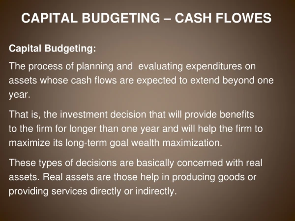
Introductory Definitions • Capital budgeting: • The process of identifying, evaluating, selecting, and controlling capital investments • Capital investments: • Long-term investment opportunities involving substantial initial cash outlays followed by a series of future cash returns • Capital budget: • Part of the organization’s master budget (Chap. 8) that deals with the current period’s planned capital investment outlays
Introductory Definitions (continued) • Discounted cash-flow (DCF) decision models: • Decision models (e. g., NPV and IRR) that explicitly incorporate the time-value-of-money • Weighted-average cost of capital (WACC) • Under normal circumstances, the discount factor used in DCF capital budgeting decision models • A weighted average of the cost of obtaining capital from various sources (e.g., equity and debt) • Non-discounted cash flow decision models: • Capital budgeting decision models that do not incorporate the time-value-of-money into the analysis of capital investment projects
How Accounting Can Add Value to the Capital Budgeting Process • Linking capital budgeting to the master budgeting process (planning) • Linking capital budgeting decisions to the organization’s Balanced Scorecard (control) • Generation of relevant data for investment analysis purposes (decision making) • Conducting post-audits (control)
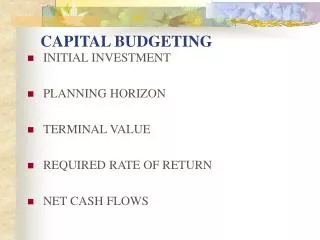
Identifying Relevant Cash Flows for Capital Expenditure Analysis • Project initiation: • Required investment outlays, including installation costs • Includes incremental net working capital commitments • Project operation: • Cash operating expenses, net of tax • Additional net working capital requirements • Operating cash inflows, net of tax • Project disposal: • Net of tax investment disposal • Recapture of investment in net working capital
Decision Example Smith Company manufactures high-pressure pipe for deep-sea oil drilling. The firm is considering the purchase of a milling machine.
Project Initiation: Net After-tax Cash Inflow, Disposal of Old Asset • Net proceeds = Selling price – Disposal costs • For gain situation: • Net cash inflow = Net proceeds – (Gain on disposal x t) • For loss situation: • Net cash inflow = Net proceeds + (Loss on disposal x t)
Smith Company Data: After-tax Cash Inflow, Disposal of Old Asset
Project Operation: After-tax Cash Operating Receipts/Savings TransactionEffect on Cash Flow Cash receipts Amount received × (1 - t) Cash expenditures Amount paid × (1 - t) Depreciated initial cost Tax shield: Depreciation expense ×t Allocated costs No effect The company expects its investment to bring in $1,000,000 in cash revenue from increases in production volume in each of the next four years. Cash operating expenses are expected to be $750,000/year.
Smith Company: After-tax Cash Operating Receipts/Savings Thus, after-tax cash from operations increases by $194,000/year ($150,000 + $44,000)
Determining the Annual Depreciation Tax Shield For simplicity, the preceding example calculated depreciation expense using the SL method. In most instances, however, companies use the Modified Accelerated Cost Recovery (MACRS) method to determine depreciation expense for tax purposes.
Smith Company: Project Disposal • The company plans to sell the machine at the end of its useful life for $100,000 and incur removal and cleanup costs of $20,000 • Return of net working ($200,000) originally invested in year 0 • At the end of the project’s life, the company will incur an estimated cost of $150,000 in relocation costs for displaced workers. This amount is fully deductible for tax purposes.
Smith Company: Projected Cash Flows--Summary Note--Not discussed previously: $50,000 (pre-tax) training costs estimated for Year 1
Additional Measurement Issues • Inflation? • Opportunity costs? • Sunk costs? • Allocated overhead costs?
Calculating the Discount Rate (WACC) • The weighted average cost of capital (WACC) is used in capital budgeting to discount future anticipated cash flows back to present-dollar equivalents • Weights can be determined based on the target capital structure for the firm or based on the current market values of the various sources of funds
Calculating the Discount Rate (WACC) (continued) • The after-tax cost of debt = Effective interest rate on debt x (1 – t) • Cost of common equity is equal to the expected/required market rate of return on the company’s stock (for listed companies, can be estimated using the CAPM)
Example: Calculating the Discount Rate (WACC) A firm has a $100,000 bank loan with an effective interest rate of 12%; $500,000, 10%, 20-year mortgage bonds selling at 90% of face’ $200,000, 15%, $20 noncumulative, noncallable preferred stock with a total market value of $300,000; and 10,000 shares of $1 par common stock. The estimated required rate of return on the common stock, based on application of the CAPM, is 20%. The firm is subject to a 40% tax rate. Let’s calculate the weighted average cost of capital...
Example: Calculating the Discount Rate (WACC) (continued) Note: the cost of preferred stock is equal to the current dividend yield on the stock, that is, current dividend per share of preferred stock current market price per share.
Class problem To illustrate, assume the Foxborough Corporation has the following financing structure: 10% Bonds $150,000 8% Preferred stock 50,000 Common stock offering a 12% return 200,000 Retained earnings with a 14% return 100,000 Total $500,000 To compute the weighted average cost of capital, find the relative percentages for each type of securities and multiply these percentage by the return offer and sum the result
Class problem Debt financing .030 Preferred stock .008 Common stock .048 Retained earnings .028 Total .114 = 11.4%
NPV Decision Model • Discount all future net-of-tax cash inflows to present value using the WACC as the discount rate • Discount all future net-of-tax cash outflows to present value using the WACC as the discount rate • If NPV > 0, accept the project (that is, the project adds to the value of the company) • If NPV < 0, reject the project (that is, the project does not add value to the company)
(1 + 10%)-1 NPV: Smith Company (@ 10.0%)
Internal Rate of Return (IRR) Model • IRR represents an estimate of the “true” (i.e., “economic”) rate of return on a proposed investment project • IRR is calculated as the rate of return that produces a NPV of zero • If IRR > WACC, then the proposed project should be accepted (i.e., its anticipated rate of return > the cost of invested capital for the firm) • If IRR < WACC, the proposed project should be rejected (i.e., its NPV will be < 0)
Estimating the IRR of a Project • General Solution: • Use built-in function in Excel When Future Cash Inflows are Uniform: • Use annuity table to identify, in the row corresponding to the life of the project, an amount = initial investment outlay annual net-of-tax cash inflow When Future Cash Inflows are Uneven: • Use a “trial-and-error” approach (with interpolation)
Sensitivity Analysis • NPV and IRR models provide an investment recommendation—accept or reject a given project • Sensitivity analysis refers to the sensitivity of the recommendation to estimated values for the variables in the decision model • “What-if” analysis • Scenario analysis • Monte Carlo simulation analysis
“What-if” Analysis Involves changing one variable (e.g., the discount rate) at a time; as part of this form of sensitivity analysis we might consider the: • Most optimistic case • Most pessimistic case • Break-even after-tax cash flow amount (use “Goal Seek” option in Excel)
Other Capital Budgeting Decision Models: Payback Period • Payback period = length of time (in years) needed to recover original net investment outlay • When after-tax cash inflows are expected to be equal, the payback period is determined as: Total initial investment/Annual after-tax cash inflows
Investment Decision Example A four-year project requires an initial investment of $555,000 in Year 0. The project is expected to produce $900,000 in cash revenues and require $660,000 in cash expenses each year. No additional working capital is required and the investment will have a salvage value of $60,000. At the end of the fourth year management expects to sell the investment for $200,000. Expected relocation costs are $240,000 and the company is subject to a 40% tax rate.
Total Original Investment Annual Net After-Tax Cash Inflow Payback Period = Investment Decision Example: Payback Calculation $555,000 $193,500 Payback Period = Payback Period = 2.87 years
Strengths of the Payback Decision Model • Easy to compute • Businesspeople have an intuitive understanding of “payback” periods • Payback period can serve as a rough measure of risk—the longer the payback period, the higher the perceived risk
Weaknesses of the Payback Decision Model • The model fails to consider returns over the entire life of the investment • In its unadjusted state, the model ignores the time value of money • The decision rule for accepting/rejecting projects is ill-defined (ambiguous) • Use of this model may encourage excessive investment in short-lived projects
Present Value Payback Model Present value payback = the amount of time, in years, for the time-adjusted (i.e., discounted) future cash inflows to cover the original investment outlay Note: if the discounted payback period is less that the life of the project, then the project must have a positive NPV
Present Value Payback Model (continued) • Strength: • Takes into consideration the time value of money • Weaknesses: • Can motivate excessive short-term investments • Returns beyond the payback period are ignored • Decision rule for project acceptance is ambiguous/subjective
Example: Calculating the Present Value Payback Period Present Value Payback Period = 3 years + ($73,794 ÷ $132,163) = 3.56 years
Accounting Rate of Return (ARR) ARR = Average annual accounting income Average investment
Accounting Rate of Return $69,750$307,500 = = 22.68% Example: Calculating ARR
Evaluation of ARR Decision Model • Advantages: • Readily available data • Consistency between data for capital budgeting purposes and data for subsequent performance evaluation • Disadvantages: • No adjustment for the time value of money (undiscounted data are used) • Decision rule for project acceptance is not well defined • The ARR measure relies on accounting numbers, not cash flows (which is what the market values)
Behavioral Issues • Cost escalation (escalating commitment)--decision makers may consider past costs or losses as relevant • Incrementalism (the practice of choosing multiple, small investments) • Uncertainty Intolerance (risk-averse managers may require excessively short payback periods) • Goal congruence (i.e., the need to align DCF decision models with models used to subsequent financial performance)
P20-38 a. Unadjusted Payback Period: As shown above, the payback period occurs between years 4 and 5. Alternatively, the payback period = $500,000 $120,000/year = 4.17 years(about 4 years and 2 months) b. Book (accounting) rate of return: As indicated above, the average increase in net income over the ten- year period = $700,000/10 years = $70,000/year. Thus, the ARR (1) On initial investment: $70,000/$500,000 = 14.00% (2) On average investment: Average investment: ($500,000 + 0)/2 = $250,000 Book rate of return: $70,000 $250,000 = 28.00% c. NPV: using the PV factors from Table 2 (p. 871), NPV = $178,120
P20-41 1. Depreciation per year, SL basis: ($30,600 – $600)/6 years = $5,000 Taxable income $8,000 – $5,000 = 3,000 Tax rate x 40% Income taxes $1,200 Pre-tax annual cash flow (cash savings) = $8,000 Net after-tax annual cash inflow: $8,000 – $1,200 = $6,800 2. Payback period: $30,600/$5,000 = 6.12 years (if cash flows are assumed to occur at end of year, then the appropriate answer would be 7 years) 3. PV of annual after-tax cash savings $5,000 x 4.623 = $23,115 PV of salvage value $ 600 x 0.63 = 378 Total Present Value of Cash Inflows $23,493 Initial Investment Cash Outlay 30,600 NPV ($7,107)
Review _______________ is a long-term project that involves a large sum of funds and that provides expected future benefits. A) A balanced scorecard B) A master budget C) A capital budget D) A capital investment E) A multicriteria decision model
Review Which of the following is NOT a contribution that the accountant makes to the capital budgeting process? A) Linkage to master budget (planning) B) Linkage to the balanced scorecard (control) C) Generation of relevant data for investment analysis purposes (decision making) D) Conducting of post-audits (control) E) All of the above are contributions made by the accountant.