Ray Tracing 2
Ray Tracing 2. Today. Anti-aliasing Surface Parametrization Soft Shadows Global Illumination Path Tracing Radiosity Exercise 2. Sampling. Ray Casting is a form of discrete sampling. Rendered Image: Sampling of the ground Truth at regular intervals. Ground Truth:

Ray Tracing 2
E N D
Presentation Transcript
Today • Anti-aliasing • Surface Parametrization • Soft Shadows • Global Illumination • Path Tracing • Radiosity • Exercise 2
Sampling Ray Casting is a form of discrete sampling. Rendered Image:Sampling of the groundTruth at regular intervals Ground Truth: An Exact MathematicRepresentation Signal Frequency? Sampling Frequency?
Anti-Aliasing Aliasing: A distortion or artifact as a result of sampling. • Higher frequency removal To reproduce the signal fully - Nyquist rate Signal Sampled • Related problem – Moiré
Anti-Aliasing • Staircasing Pixels on the boundary
Anti-Aliasing • Anti-aliasing - The attempt to reduce or eliminate aliasing artifacts
Uniform Supersampling • Instead of sampling one point in every pixel. Sample k2times (for some n) in uniform intervals • Set the pixel color to the average of the k2colorssampled Single Pixel - Multiple Sample Single Pixel - Single Sample
Cast ray through pixel • Constructing a ray through a pixelParameters: • Eye point – P • View direction - towards • Up direction • Field of view – (xfov, yfov) • Distance to screen – d right = towards x up right and up define theorientation of the screen. P0 and d define where it’s at. xfov center of screen Pc yfov d up towards P0 right
Cast ray through pixel Pc = P0 + towards*d P is the pixel at (xpixel, ypixel) = (2, 2) Calculate (xscreen, yscreen) P = Pc + xscreen*right + yscreen*up V = (P - P0) / ||P - P0|| ray direction to P. xfov P up Pc right yfov d V towards ray = P0 + t*V P0
Cast ray through pixel • Transforming (xpixel, ypixel) to (xscreen, yscreen) pixel-width = 320 px xfov = 2.0 +x +y +up yfov = 2.0 Pc +right pixel-height = 240 px Screen – In Object Space Application Window
Uniform Supersampling Pixel coordinates can now have fractions Pc = P0 + towards*d P is the pixel at (xpixel, ypixel) = (2.5, 2.5) Calculate (xscreen, yscreen) P = Pc + xscreen*right + yscreen*up V = (P - P0) / ||P - P0|| ray direction to P. do this k2 times, average results. xfov P up Pc right yfov d V ray = P0 + t*V towards P0
Uniform Supersampling 1 sample per pixel Where should you sample the pixel? 0 ½ 1 1 0 ½ ¼ ¾ 0 0 4 sample per pixel ¼ ½ ½ ¾ 1 1 9 sample per pixel
Uniform Supersampling • Global uniformity:Distance betweenSamples is always the same • What NOT to do: Two samples in the same point
Adaptive Supersampling If the difference between adjacent samples is too great, divide the pixel to 4 and cast more rays • Smooth pixels need only 4 samples • Edges can still be reproduced smoothly • Reuse common rays
Stochastic Sampling • Uniform sampling often still can’t account for frequency issues • Sub-divide the pixel to a grid • Choose a random point in every cell • Makes the interval of sampling non-uniform • Reduce aliasing by introducing noise
Surface Parameterization How to add a 2D texture to a surface embedded in 3D? (x,y,z)
Surface Parameterization P4 P3 Simple case – rectanglular plane u P v P1 P2 u [0,1], v [0,1] P = -v * (P3-P1) + u * (P2-P1) Baricentric coordinates Equation 1. Extract (u,v) from P 2. Get the pixel color at (u,v)
Surface Parameterization P4 P3 Simple case - rectanglular plane u P v P1 P2 u [0,1], v [0,1] P = -v * (P3-P1) + u * (P2-P1) Baricentric coordinates Equation 1. Extract (u,v) from P 2. Get the pixel color at (u,v)
Surface Parameterization P A Little more complex - Sphere u v P = (x,y,z) (,,r) • u =, v = Sphertical Coordinates u [0,1], v [0,1] 1. Extract (u,v) from P 2. Get the pixel color at (u,v)
Surface Parameterization General Case – A Triangle Mesh
Surface Parameterization P A Little more complex - Sphere u v P = (x,y,z) (,,r) • u =, v = Sphertical Coordinates u [0,1], v [0,1] 1. Extract (u,v) from P 2. Get the pixel color at (u,v)
Area Light • So far we’ve see only “ideal” light sources • Light from infinity • Point Light • Spot Light • These produce“Hard Shadows” • To Create a realisticShadow one option isto use a morerealistic light source Directed Light Point Light Area Light
Area Light • Point light - Hard Shadows Lighs Source Full Shadow Umbra
Area Light • Simple area light - simulated using a uniform grid of point lights. Lighs Source Full Shadow Umbra Soft Shadow Penumbra
Area Light • Disadvantages of the simple uniform method: • Very time consuming • If the grid resolution is low, artifacts appear in the shadows.
Area Light Monte-Carlo Area light • Light is modeled as a sphere • Highest intensity in the middle. Gradually fade out. • Shoot n rays to random points in the sphere • Average their value.
Monte Carlo vs Las Vegas • Two types of randomized, probabilistic methods for constructing an algorithm • Results are statistic – Has an expectancy E(X) to be correct. • Monte Carlo: • Has a predictable time complexity. • Result may not be correct. • Better results the more you run it • Las Vegas: • Time complexity not guaranteed • Always returns the correct answer • Convert Monte-Carlo to Las-Vegas?
Global Illumination In the real world light is everywhere. • Reflects in every direction from every surface onto every surface. • Anywhere in the world, light comes from infinite directions around. In the lighting equation we’ve used the Ambient intensity to approximate this.
Monte-Carlo Path Tracing • Conventional Ray Tracing: • Cast rays from eye through each pixel • Trace secondary rays to light sources and reflections
Monte-Carlo Path Tracing • A generalization of the concept of Monte-Carlo area light • Cast rays from eye through each pixel • Cast random rays from the visible point, average contributions
Monte-Carlo Path Tracing • Cast rays from eye through each pixel • Cast random rays from the visible point, average contributions • Recurse
Monte-Carlo Path Tracing • Cast rays from eye through each pixel • Cast random rays from the visible point • Recurse, accumulate contributions
Monte-Carlo Ray Tracing • Cast random rays from the visible point • Recurse, accumulate contributions • Sample light from all points we visited
Monte-Carlo Path Tracing 1 random ray per pixel, 1 level recursion
Monte-Carlo Path Tracing 16 random rays per pixel, 3 level recursion
Monte-Carlo Path Tracing 64 random rays per pixel, 3 level recursion
Monte-Carlo Path Tracing 64 random rays per pixel, 3 level recursion NoticeColor Bleed To White ball
Monte-Carlo Path Tracing 16 random rays per pixel1 level recursion 16 random rays per pixel100 level recursion
Glossary • Ray Casting: • Cast rays from eye through each pixel, find first hit • Ray Tracing: • Cast rays from eye through each pixel, find first hit • Recourse- Ray changes course/divides into few rays • Accumulate all results. • Path Tracing • Cast rays from eye through each pixel, find first hit • Recourse- Shoot random rays in the reflect hemisphere • Accumulate All results 1-3 rays per recursion step 1-100 rays per recursion step
Glossary • Direct Illumination • Find a interaction between objects and emitters of light • “How much light from light source X hits this point” • Ray Tracing • Global Illumination • Find interaction between objects and complete environment • “How much light hits this point”, “Indirect lighting” • Path Tracing • Faked with The Ambient constant in the light equation. • Radiosity • Photon mapping
Radiosity(simplified) • A different approach to Global Illumination • Divide the scene into a set of small areas • The radiosicy of a patchis the total amount of lightemitted from it • Calculate all the amountof light a patch receives fromall other patches. • Calculate the radiosity • Iterate.
Radiosity Calculating the amount of light a patch receives • Construct a “Hemicube” on the patch • Render the scene on the hemicube • Average the color.
Radiosity Rendering on a hemicube
Radiosity Light emitted = Color * Light received Initial State First Iteration
Radiosity Compute light emissions once, View from any angle! 32nd iteration 320th Iteration
Radiosity Direct Illumination Radiosity
Radiosity – Surface Subdivision • Using a uniform mesh? • Wasteful. Smooth areas don’t need a great level of detail • Hierarchical subdivision • Areas with large changes get subdivided.