Download

1 / 15
150 likes | 270 Vues
This regression-based approach by Dr. Sunil Maheshwari from Dominion Virginia Power offers benefits for both weather-sensitive and non-weather-sensitive loads. The method involves estimating the load based on various factors like weather, time, and day of the week, using established functional forms to ascertain the best fit. By applying the theory to practice, precise load predictions are achieved, with equations easily updatable annually. Utilizing regression analysis enhances accuracy in load forecasting.

E N D
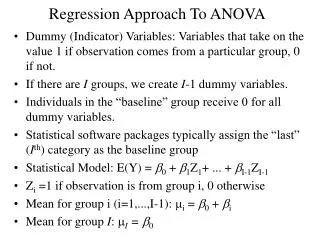
Regression-based Approachfor Calculating CBL Dr. Sunil Maheshwari Dominion Virginia Power
Benefits of Regression Approach • This approach can be used to calculate CBL for both weather-sensitive and non-weather-sensitive loads. • The science of regression theory is well developed. • Most statistical packages such as SAS, STATA, SPSS, etc. can perform regression analysis. • Regression equations can be easily updated on a periodic basis (perhaps annually).
Description of Regression Approach • The idea is to treat load as a function of explanatory factors such as weather, time of day, day of the week, etc. • Estimate the relationship between load and explanatory variables using a variety of functional forms. • Pick the functional form that gives the highest R-sq adjusted or the lowest Root Mean Squared Error (RMSE)
Functional Forms for Weather-Sensitive Loads Form 1: Load = a + b*CDD + c*HDD Form 2: Load = a+ Σ (bi * CDDi) + Σ (cj * HDDj); Temperature breakpoints to be established based on Regression Analysis Form 3: Load = a+ Σ (bi * CDDi) + Σ (cj * HDDj) + Σ (dk * hourk); In addition to weather, each hour impacts the load as well.
Functional Forms for Non-Weather Sensitive Loads • The following forms may do a good job of estimating CBL for Industrial loads: Form 4: Load = a + Σ (bk * hourk) + Σ (cj * monthj); Form 5: Load = a + b * TimeTrend + Σ (ck * hourk) + Σ (dj * monthj);
Applying Theory into Practice… • For one of our DSR participants (a Building Complex), we estimated the relationship between 2006 hourly Load and Weather using Functional Form 3: Load = a+ Σ (bi * CDDi) + Σ (cj * HDDj) + Σ (dk * hourk); • Following temperature breakpoints were used: • For Heating Degree Days (HDD) – 65, 55, 40, 25 • For Cooling Degree Days (CDD) – 65, 80, 90, 100
Applying Theory into Practice… • We further sliced the data by: • Day type • Weekdays • Weekends and Holidays • Season • Winter – December - March • Summer – June - September • Shoulder – April, May, October, November
Partial Regression Output (Summer, Weekday) regress load cdd_65to80 cdd_80to90 cdd_90to100 cdd_over100 hdd hddsq hour2-hour24 if year==2006 & weekdayflag==1 & holiday==0 & season=="Summer" Source | SS df MS Number of obs = 2040 -------------+------------------------------ F( 28, 2011) = 518.86 Model | 339127510 28 12111696.8 Prob > F = 0.0000 Residual | 46942715.2 2011 23342.9713 R-squared = 0.8784 -------------+------------------------------ Adj R-squared = 0.8767 Total | 386070225 2039 189342.925 Root MSE = 152.78 ------------------------------------------------------------------------------ load | Coef. Std. Err. t P>|t| [95% Conf. Interval] -------------+---------------------------------------------------------------- cdd_65to80 | 33.08646 .9634143 34.34 0.000 31.19707 34.97586 cdd_80to90 | 31.6024 .5931229 53.28 0.000 30.4392 32.7656 cdd_90to100 | 32.58845 .68489 47.58 0.000 31.24528 33.93162 cdd_over100 | (dropped) hdd | -104.137 6.194134 -16.81 0.000 -116.2846 -91.98941 hddsq | 4.866126 .6342737 7.67 0.000 3.622224 6.110028 hour2 | -33.26744 23.44299 -1.42 0.156 -79.24253 12.70765 hour3 | 19.0973 23.452 0.81 0.416 -26.89547 65.09006 hour4 | 25.50128 23.46632 1.09 0.277 -20.51955 71.52211
Predicted Load (CBL) based on 2006 data applied to 2007 data • Using regression parameters from previous slide, predict the load for 2007. • Compare predicted load (CBL) to actual load. • Absolute average % deviation between Actual and Predicted Load was less than 5%. • Regression Equations will be re-estimated every year
Actual Load vs Predicted (CBL) - Summer, Weekday(Absolute Average % Deviation = 3%)
Actual Load vs Predicted (CBL) - Winter, Weekday(Absolute Average % Deviation = 3.6%)
Actual Load vs Predicted (CBL) - Shoulder, Weekday(Absolute Average % Deviation = 3.7%)
Actual Load vs Predicted (CBL) - Weekend/Holiday(Absolute Average % Deviation = 4.7%)
Conclusions • 4 Equations with single variable hourly temperature • Summer, Weekday • Winter, Weekday • Shoulder, Weekday • Weekends / Holidays • Good fit (R-sq adjusted > 78% in all cases). • Simplified calculations, and the regression equations can be easily updated.