Download
1 / 1
10 likes | 127 Vues
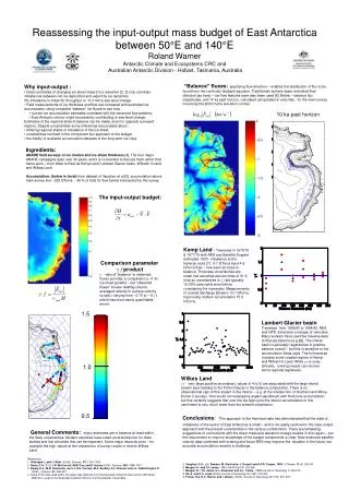
Reassessing the input-output mass budget of East Antarctica between 50°E and 140°E Roland Warner Antarctic Climate and Ecosystems CRC and Australian Antarctic Division - Hobart, Tasmania, Australia.

E N D
Reassessing the input-output mass budget of East Antarctica between 50°E and 140°ERoland WarnerAntarctic Climate and Ecosystems CRC and Australian Antarctic Division - Hobart, Tasmania, Australia “Balance” fluxes: specifying flow direction – enables the distribution of flux to be found from the continuity (budget) equation. Traditionally surface slope motivated flow direction (as here) – ice flow features have also been used [6]. Below – balance flux magnitudes, and 10 ka past horizon, calculated using balance velocities, for the main survey line along the 2000 metre elevation contour. • Why input-output : • Direct estimates of changing ice sheet mass [1] or elevation [2, 3] only constrain imbalances between net ice deposition and export by ice dynamics. • 5% imbalance in Antarctic throughput is ~0.3 mm/a sea-level change. • Field measurements of ice thickness and flow are compared with estimated ice accumulation using computed “balance” ice fluxes to see how : • current ice accumulation estimates correlates with the observed flow patterns, • East Antarctic interior might be presently contributing to sea-level change. • Estimates of the regional state of balance can be made, even for sparsely surveyed regions. Despite uncertainties some inferences are possible about : • differing regional states of imbalance of the ice sheet, • uncertainties involved in the component flux approach to the budget • the fidelity of available accumulation datasets to the long-term ice input. 10 ka past horizon Ingredients: ANARE field surveys of ice motion and ice sheet thickness [4]. The four major ANARE campaigns span over 30 years, and it is convenient to discuss them within that frame-work – from West to East as Kemp Land, Lambert Glacier basin, Wilhelm II Land and Wilkes Land. Accumulation: (below in (m/a)) from dataset of Vaughan et al [5]. accumulation above main survey line ~225 GTon/a - 46 % of total for flow bands intersected by the survey. The input-output budget: Kemp Land - Traverses in 1975/76 & 1977/78 with RES and Satellite Doppler estimated 100% imbalance at the traverse route [7] : 9.1 GTon/a input 4.6 GTon/a flow – now seen as close to balance. Thickness uncertainties are small, but velocities are low (max of 31.8 m/a) so uncertainties in gf are typically 10-20% (see right) even before considering the numerator. Measurements of coastal discharge [8] were 10.1 GTon/a. Input using modern accumulation 15.9 GTon/a. Comparison parameter gf product g - ratio of “balance” to observed fluxes provides a comparator (g >1 for ice sheet growth) – but “observed fluxes” involve relating column-averaged velocity to surface velocity (a ratio f varying from ~0.75 to ~1) g f which has more easily quantifiable errors. 1.5 Lambert Glacier basin Traverses from 1989/90 to 1994/95. RES and GPS. Extensive coverage of velocities. Many workers have used the traverse data to discuss balance (e.g.[9]). The interior basin is generally regarded as in positive balance overall – but this is sensitive to the accumulation fields used. The full traverse includes some coastal regions in Kemp and Wilhelm II Land. While gf is noisy (shown), running means can recover some regional signatures. 1.0 Wilkes Land g f - very large positive anomalies ( values of 4 to 5) are associated with the large inland stream seen leading to the Totten Glacier in the balance computation. There is no observational sign of this stream in the interior – e.g. at the intersection of Southern and Mirny-Dome C surveys. One would not necessarily expect equilibrium with Holocene accumulation but this certainly suggests that over the Ice Age cycle the interior accumulation in this catchment is very much lower than the present compilation. Conclusions:This approach to the historical data has demonstrated that the state of imbalance of this sector of East Antarctica is small – and is not easily resolved in the input-output approach with the present uncertainties in the various contributions. There are tantalising suggestions of connections with the direct mass and elevation change studies in this region – but the requirement to improve knowledge of the budget components is clear. New extensive satellite velocity data combined with existing and future RES may improve the situation in the future, but accurate accumulation remains a challenge. 0.5 General Comments: many estimates are in balance at least within the likely uncertainties. Modern velocities have small uncertainties but for older studies and low velocities this can be important. Some major discords exist – for example the high values at the intersection of survey routes in interior Wilkes Land. References: 1 Velicogna I., and J. Wahr, (2006), Science, 311,1754-1756. 2 Davis, C.H., Y. Li, J.R. McConnell, M.M. Frey and E. Hanna (2005). Science, 308, 1898–1901. 3 Zwally, H.J., M.B. Giovinetto, Jun Li, H.G. Cornejo, M.A. Beckley, A.C. Brenner and J.L. Saba Donghui Yi (2005). J Glaciol, 51, 509-527. 4 Some of the data used within this paper was obtained from the Australian Antarctic Data Centre (IDN Node AMD/AU), a part of the Australian Antarctic Division (Commonwealth of Australia). . 5 Vaughan, D.G., J.L. Bamber, M. Giovinetto, J. Russell and A.P.R. Cooper, 1999, J Climate, 12 (4), 933-94 6 Morgan V.I. and T.H. Jacka, (1981) IAHS Publ131,253-260 7 Morgan V.I., T.H. Jacka, G.J. Ackerman and A.L. Clarke, (1982) Annals of Glaciology 3, 204-210 8 Wu X. and K.C. Jezek (2004) Journal of Glaciology 50 (169), 219-230 9 Fricker H.A, R.C. Warner and I. Allison, (2000), Journal of Glaciology 46 (155). 561-570;