The plan for today
The plan for today. Camera matrix Part A) Notation, preprocessing, and basic concepts. Part B) 4 Stereo Algorithms. Slides are courtesy of Prof. Ronen Basri . Stereo Vision. Objective: 3D reconstruction Input: 2 (or more) images taken with calibrated cameras

The plan for today
E N D
Presentation Transcript
The plan for today • Camera matrix • Part A) Notation, preprocessing, and basic concepts. • Part B) 4 Stereo Algorithms Slides are courtesy of Prof. Ronen Basri
Stereo Vision • Objective: 3D reconstruction • Input: 2 (or more) images taken with calibrated cameras • Output: 3D structure of scene • Steps: • Rectification • Matching • Depth estimation
Rectification • Image Reprojection • reproject image planes onto common plane parallel to baseline • Notice, only focal point of camera really matters (Seitz)
Rectification • Any stereo pair can be rectified by rotating and scaling the two image planes (=homography) • We will assume images have been rectified so • Image planes of cameras are parallel. • Focal points are at same height. • Focal lengths same. • Then, epipolar lines fall along the horizontal scan lines of the images
Cyclopean Coordinates • Origin at midpoint between camera centers • Axes parallel to those of the two (rectified) cameras
Disparity • The difference is called “disparity” • dis inversely related to Z: greater sensitivity to nearby points • dis directly related to b: sensitivity to small baseline
Main Step: Correspondence Search • What to match? • Objects? More identifiable, but difficult to compute • Pixels? Easier to handle, but maybe ambiguous • Edges? • Collections of pixels (regions)?
Random Dot Stereogram • Using random dot pairs Julesz showed that recognition is not needed for stereo
1D Search • More efficient • Fewer false matches SSD error disparity
Finding Matches • Under what conditions pixels can be matched? • Ignoring specularities, we can assume that matching pixels have the same brightness (constant brightness assumption) • Still, changes in gain and sensitivity may change the values of pixels
Possible solutions • Use larger windows • Constraint the search • Other metric e.g., Normalized correlation
Window Size W = 3 W = 20
Constraining the Search • Restrict search to epipolar lines (1D search) • Enforce ordering Problem: not always true • Enforce smoothness Problem: discontinuities at object boundaries
Summary basic ideas • Restrict search to epipolar lines (1D search) • Use larger elements (larger windows, edges, regions) Problem: large elements may be distorted • Enforce ordering Problem: not always true • Other similarity measures (e.g., Normalized correlation) • Enforce smoothness Problem: discontinuities at object boundaries
Comparison of Stereo Algorithms D. Scharstein and R. Szeliski. "A Taxonomy and Evaluation of Dense Two-Frame Stereo Correspondence Algorithms," International Journal of Computer Vision,47 (2002), pp. 7-42. Scene Ground truth
Results with window correlation Window-based matching (best window size) Ground truth
Graph Cuts Graph cuts Ground truth
Correspondence as Optimization • Most stereo algorithms attempt to minimize a functional that usually consists of two terms: where - penalizes for quality of a match (unary) - penalizes non smooth (or even non fronto-parallel) reconstructions (binary) • Many different optimization approaches were proposed
Part B) 4 Stereo Algorithms • Dynamic programming • Minimal cut/Max flow • Space carving • Graph cut optimization
1D Methods: Dynamic Programming • Discretize the 3-D space • Find the correct curve at every slice (A slice = epipolar plane)
Dynamic programming Find correspondences of each epipolar line separately
Dynamic programming How do we find the best curve? • Assign weight of all edges insertion match deletion
Dynamic programming How do we find the best curve? • Assign weight of all edges • Find shortest path • Dijkstra insertion match deletion
Dynamic programming Advantages • Simple, efficient • Globally optimal Disadvantages • Each slice computed independently (smoothness is not enforced between slices) • Problems due to discretization (tilted planes)
Stereo Algorithms Brief review of 4 algorithms: • Dynamic programming • Minimal cut/Max flow • Space carving • Graph cut optimization
Min Cut/Max FlowMain idea: Lets solve all DP problem together. Objective: find the optimal cut using all the slices simultaneously.
Min Cut/Max Flow Construct a graph: • Every voxel (3-D point in space) is a node • Every node is connected to its 6 neighbors
Min Cut/Max Flow Weights on the edges: • Data cost: change in pixel value Neighbor Innext slice/row data Neighbor Neighbor data Neighbor Innext slice/row
Min Cut/Max Flow Weights on the edges: • Data cost: change in pixel value • Smoothness cost: change in depth smooth smooth smooth smooth
Min Cut/Max Flow Weights on the edges: • Data cost: change in pixel value • Smoothness cost: change in depth data
… … Min Cut/Max Flow Source • Add source and sink • Find min cut ∞ ∞ Sink
Min Cut/Max Flow Data penalty Smoothness penalty
Results Input Min cut Dynamic programming
Min Cut/Max Flow Advantages • All slices are optimized simultaneously • Efficient Disadvantages • Extension to multi-camera is difficult • Discretization
Space Carving • Multi-view stereo • Every point in space corresponds to a match in the images • Compute data term for each match
Space Carving • Multi-view stereo • Every point in space corresponds to a match in the images • Compute data term for each match (“photo-consistency”)
Space Carving • Dynamic data term (taking occlusion into account) • Order of sweep is important