Download
1 / 50
500 likes | 602 Vues
What Can the Atmospheric Emitted Radiance Interferometer (AERI) Tell Us About Clouds?. Dave Turner SSEC / University of Wisconsin - Madison CIMSS Seminar 9 Nov 2005. Motivation to Study Clouds with Low LWP.

E N D
What Can the Atmospheric Emitted Radiance Interferometer (AERI) Tell Us About Clouds? Dave Turner SSEC / University of Wisconsin - Madison CIMSS Seminar 9 Nov 2005
Motivation to Study Clouds with Low LWP • Solar and infrared radiation is most sensitive to changes in cloud optical depth at low optical depths • ISCCP results show mean LWP for low level clouds is 51 g m-2 (Rossow and Schiffer 1999) • Over 50% of the warm liquid water clouds at the SGP site have LWP < 100 g m-2 (Marchand et al. 2003) • Over 80% of all liquid-bearing clouds observed during SHEBA have LWP < 100 g m-2 (Shupe and Intrieri 2004) • Over 90% of the non-precipitating liquid clouds over Nauru have LWP < 100 g m-2 (McFarlane and Evans 2004) • Uncertainty in the LWP observed by 2-channel microwave radiometers (23 & 31 GHz) is (at least) 20-30 g m-2 (i.e., errors of 20% to over 100%) • Implications for • Earth energy balance • Understanding cloud processes • Aerosol indirect effect
Radiative Flux Sensitivity Atmos Tropical MLW Eff. Radius 6 µm: Solid 12 µm: Dashed
LWP Frequency Distribution for Warm (> 5°C) Clouds at SGP Temperature from sonde Mode: 40 g/m2 Median: 93 g/m2 % below 100 g/m2: 53% Jan – Dec 1997 Temperature from IRT Mode: 85 g/m2 Median: 142 g/m2 % below 100 g/m2: 33% From Marchand et al., JGR, vol 108, 2003
Uncertainty in the ARM MWR’s Statistical Retrieval of LWP • PDF of LWP using the statistical retrieval during clear sky periods from 1996 – 2001. • Clear sky periods were classified as such if the MMCR and lidar did not detect any cloud for a 3-hr period • Doesn’t include any systematic biases! From Marchand et al., JGR, 2003
Spread of 40 g/m2 Understanding the Accuracy of the MWR’s LWP: Different Methods, Different Results • 1 Set of MWR Tb observations • 4 different submissions • 3 different retrieval methods • 4 different absorption models
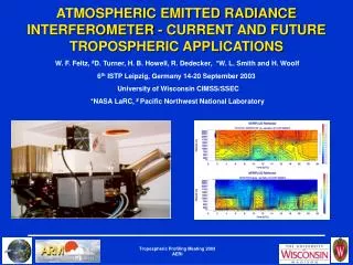
Atmospheric Emitted Radiance Interferometer (AERI) • Automated instrument measuring downwelling IR radiation from 3.3-19 µm at 0.5 cm-1 resolution • Uses two well characterized blackbodies to achieve accuracy better than 1% of the ambient radiance • Data used in a wide variety of research • Instrument details in Knuteson et al. JAM 2004 • Typically collects 3-min avg every 8 min
Location of the ARM AERIs Pt. Reyes (Mobile Facility)
Clear Sky Spectra 25 µm 15 µm 10 µm 7.1 µm
Cloudy Sky Spectra (1) Liquid water cloud at 1.0 km US Standard Atmosphere
Cloudy Sky Spectra (2) Liquid water cloud at 1.0 km US Standard Atmosphere
Atmospheric Model Assumes a single layer infinitesimally thin cloud
AERI Retrieval Method (MIXCRA) • Infrared radiance is very sensitive to cloud with the condensed water path is small (less than ~50 g/m2) • Many groups have used the 8-13 µm band to retrieve cloud properties • Algorithm developed to retrieve microphysical properties of mixed-phase clouds in Arctic • Uses observations in the 8-13 µm and 17-24 µm bands • Dual-phase retrieval only applicable for low PWV conditions (PWV < ~1 cm) • Use of optimal estimation allows algorithm to retrieve single-phase cloud properties in higher PWV conditions • Method published in Turner, JAM 2005 • Liquid-only method extended to use observations in the 3-5 µm band during daytime • Allows the retrieval of a “cloud fraction” term • Increases the range of the total cloud optical depth that can be retrieved • Improves accuracy of the effective radius retrieval • Method published in Turner and Holz, GRSL 2005
Retrieval Uncertainties • Uncertainties in observations and parameters, as well as the sensitivity of the forward model, result in uncertainties in retrieved cloud properties • Often sample/case specific • Bayesian and Optimal-Estimation techniques (and others) are excellent approaches, but can be difficult to set up problem and identify correlated errors • A couple of case studies does not replace a more robust, point-by-point, uncertainty estimation analysis!
Uncertainties ExampleRetrieving Optical Depth from IR Radiation • Uncertainty in PWV has a variable impact on the cloud emissivity (i.e., cloud optical depth) • Impact is a function of cloud temperature
Jacobian Observation A priori Forward model State vector A priori’s Covariance “Obs” Covariance A Word About Optimal Estimation • Technique is an old one, with long history • Excellent book by Rodgers (2000) • Many good examples exist in literature • Assumes problem is linear and uncertainties are Gaussian • However, the accuracies of the uncertainty in X is directly related to ability to properly define the covariance matrix of the observations Sε, which is a non-trivial exercise • Key advantage is that uncertainties in the retrieved state vector X are automatically generated by method !
Calculating the Observation Covariance Matrix Sε • Observed variable is downwelling radiance • Sources of uncertainty: • Clear sky radiance (primarily driven by PWV) • Cloud temperature • Instrument noise • Sky variance during sky dwell • Cloud single scattering properties (habit and size distribution) • Instrument noise is only source that is assumed to be uncorrelated across the spectrum • Off-diagonal elements of Sm are critical, but often ignored! • Determined in my application by using the chain-rule • Currently not capturing the uncertainty in the cloud scattering properties in my retrievals
14.3 μm 7.7 μm AERI Obs: 6 Nov 2003 at 20.258 UTC LBLDIS Calc: Taug = 6.6, reff = 1.5 μm, Fc = 82% LBLDIS Calc: Taug = 6.6, reff = 1.5 μm, Fc = 82 • Including 3-5 μm radiance during the daytime results in unique solution • However, must invoke a radiative “cloud fraction” term… 5.0 μm 3.84 μm AERI Obs: 6 Nov 2003 at 20.258 UTC LBLDIS Calc: Tau = 6.6, reff = 1.5 μm, Fc = 82% LBLDIS Calc: Tau = 3.2, reff = 2.5 μm, Fc = 100% AERI Obs: 6 Nov 2003 at 20.258 UTC LBLDIS Calc: Tau = 6.6, reff = 1.5 μm, Fc = 82% LBLDIS Calc: Tau = 3.2, reff = 2.5 μm, Fc = 100% Multiple Solutions In Thermal IR? • More than one answer possible using only thermal infrared (shown by Moncet and Clough JGR 1997) NOTE: LWP the same in both cases! Turner and Holz, GRSL 2005
TSI Cloud Images Multiple Solutions Example
TSI Cloud Images 6 Nov 2003 18:00 18:30 19:00 19:30 20:00
If only thermal band is used, then unable to retrieve optical depths above 6 so remaining mass was put into larger droplets • Using 8-13 and 3-5 μm observations gave much better agreement with Min algorithm • Retrieved Fc ~ 1 Evaluating MIXCRA6 Nov 2003 • AERI sensitive to LWPs approaching 70 g/m2 (depends on PWV) Turner and Holz, GRSL 2005
“Cloud Fraction” on 20 Apr • AERI samples sky for 3-min every 8 with ~2° FOV • Fc retrieved using both 8-13 and 3-5 μm AERI obs • Compared with 10 Hz IRT (2.5° FOV) and 10° zenith FOV from TSI • Good correlation with both high-res IRT and TSI obs Turner and Holz, GRSL 2005
Cumulus LWP comparisons on 20 Apr • Challenging to compare instruments with different FOVs and different sampling in broken clouds like cumulus • Nonetheless, averaged MWR data correlated well with LWP from MIXCRA (0.673); non-surprising bias seen • 3-min sky averages every 8-min are inadequate for Cu studies
CLOWD [Clouds with Low Optical (Liquid) Depth] • New working group in ARM • Objectives: • Characterize current retrievals of LWP and re from different approaches for LWP < 100 g m-2 for different atmospheric conditions and cloud types • Develop a robust retrieval algorithm using standard ARM to provide accurate LWP and re for all conditions • First step: Organize an intercomparison of published algorithms for a finite set of case study days • Cases include warm stratus, Cu, mid-level mixed-phase, and overlapping clouds • Article being written now, will submit to BAMS in Dec ‘05
Some Low LWP Retrievals • MWR retrievals (Clough et al. 2005, Liljegren et al. 2001, Lin et al. 2001, ARM statistical method) • Invert brightness temps at 23.8 and 31.4 GHz to get PWV and LWP • 4 different submissions, which use different retrieval methods and absorption models • MFRSR (Min and Harrison 1996) • Diffuse transmittance at 415 nm yields • Using LWP from MWR, can retrieve re • MIXCRA (Turner 2005, Turner and Holz 2005) • Infrared radiance inverted using optimal estimation technique to yield and re • Microbase (Miller et al. 2003) • Used Liao and Sassen (1994) to relate radar reflectivity to LWC and estimate re • Constrained the LWC to agree with the MWR’s LWP • VISST (Minnis et al. 1995) • Uses GOES radiance obs at 0.65, 3.9, 11, and 12 μm • 10 km diameter footprint
Overcast Stratiform Case 3/14/2000 20:30 21:00 21:30
Comparing MIXCRA and MWR LWP retrievals for marine stratiform clouds • ARM deployed its mobile facility to Pt. Reyes CA from April – September 2005 • Marine stratiform clouds with low LWP were present very frequently • Excellent opportunity to compare the MWR’s retrieved LWP with that retrieved by MIXCRA… • Note: Clear sky biases have been observed in the MWR’s retrieved LWP. Thus, ARM is pursuing a hypothesis that the clear sky bias can be subtracted, yielding improved LWPs in cloudy conditions
LWP Comparison (MIXCRA and MWR)NSA Site during M-PACE (Oct 2004) MWRRET MIXCRA-L MWR Retrievals performed before Tb offsets removed
LWP Comparison (MIXCRA and MWR) MWR Retrievals performed before Tb offsets removed
Motivation to Study High Clouds • Upper tropospheric ice clouds cover 40% of the globe on average at any given time (Liou 1986, Wylie et al. 1994) • Occur in extensive sheets covering a large area • Ice clouds tend to have smaller optical depths, reflect less incoming solar, and absorb more infrared radiation than water clouds (i.e. stratus) • High altitude tropical cirrus can play an important role in stratospheric/tropospheric exchange • Accurate cloud properties are crucial to • Improving and evaluating GCMs • Understanding the radiative feedback of high clouds on climate
Sensitivity to Ice Habit • Most ice cloud remote sensing methods are required to make some assumption on the habit (or effective density) of the ice crystals • This assumption dictates the single scattering properties of the ice crystals • Lots of work in the last decade deriving scattering properties (models) of ice crystals of different habits (bullet rosettes, hexagonal columns, plates, aggregates, droxtals, etc.) using geometric optics, FDTD, T-Matrix, anomalous diffraction approximation, etc. • Do these models accurately represent the scattering properties of real ice crystals with that shape? • Are these models consistent across the entire electromagnetic spectrum? • Do these models capture the dynamic range of ice crystal scattering in the atmosphere? • How should the vertical variability in habit be treated in passive retrievals? Or in active retrievals, for that matter?
Liquid water Habit Case Study: NSA 17 Oct 2004 CPI Observations at ~21:00 UT indicated particles were mostly bullets…
AERI Method (Turner) Habit Case Study: NSA 17 Oct 2004 Wang and Sassen Radar-Lidar DM-Bullet Rosette DM-Complex Polycrystal PY-Bullet Rosette PY-Column PY-Aggregate 80 • Habit scattering properties from P. Yang and D. Mitchell • Different sensitivities between IR and radar-lidar techniques! Radar – Lidar Method (Donovan / McFarlane) 0 80 0
Vertical Profile of Microphysics • Passive retrievals are extremely limited in ability to retrieve vertical profiles of re, IWC, etc. • Comparing active vs. passive methods, need to consider weighting functions NSA 17 Oct 2004 at 15:00 UTC Total optical depth: ~0.8 Radar-lidar re Radar-lidar extinction coef Both methods assumed bullet rosettes MIXCRA re
Example of a mixed-phase retrieval Turner, JAM 2005
SHEBA Results: Statistics Optical Depth Liquid re Ice re Mixed-phase Ice only Liquid only Turner, JAM 2005
SHEBA ResultsEffective Radius in Liquid-only Clouds • It is well known that aerosols from mid-latitudes are advected into the Arctic in the springtime • Are we looking at the 1st indirect effect of aerosols? Unfortunately, there were no routine aerosol observations during SHEBA… Turner, JAM 2005
The Need to ‘Rapid-Sample’ • Initial AERI temporal resolution: 3 min sky avg every 8 min • Selected for clear sky RT studies and thermodynamic profiling • Inadequate to capture changes in cloud properties
Another RS Example: Cumulus Rapid sample (16 s avg every 20 s, with occasional 20 s gaps) Nominal sample (3 min avg every 8 min)
AERI Noise Filter Algorithm • By reducing the averaging time of the radiance observations, more sky spectra can be collected although the random error increases proportionally • Desire to reduce the uncorrelated random error in these ‘rapid-sample’ observations • Decompose the matrix of AERI radiance obs using principal component analysis (PCA) • PCs associated with small eigenvalues are typically associated with uncorrelated random error; therefore, reconstruction of the data using a subset of PCs with largest eigenvalues will reduce the random error • Objective method is used to identify the number of PCs to use in the reconstruction • Algorithm has been extensively tested on over 6 years of data (2 years from each of the three ARM sites) • Paper detailing the method and results has been submitted to JTECH in Aug 2005
Noise Filter VAP “Teaser” • Number of PCs needed for adequate reconstruction is a function of: • Instrument – Season • Location – Instrument sampling rate
“Retrieving” Relative Number of Giant vs. Accumulation Mode Aerosol • Assume an effective radius and chemical composition • Use MIXCRA to retrieve optical depth for different ratios of number of giant mode to number of accumulation mode aerosol • Compare results with MFRSR • Infer the “correct” ratio of giant vs accumulation mode aerosol
Summary • Optically thin clouds (both water, ice, and mixed-phase) occur frequently in nature • AERI radiances can be inverted to retrieve cloud water path, effective radius, optical depth (and if PWV is low enough, phase) • AERI-retrieved cloud properties are being used to investigate: • Biases & sensitivity of MWR retrievals of LWP • Properties of cumulus and marine stratus • Properties of mixed-phase clouds (Arctic and mid-lat) • Consistency of ice single scattering property models • Important input to large ARM effort to compute broadband heating rate profiles to use in SCM & CRM evaluation • Information about the coarse mode aerosols, including their composition