Forecasting for Operations
Forecasting for Operations. Everette S. Gardner, Jr. Forecasting for operations. Research themes The damped trend Case studies Supply chain costs: Specialty chemicals Manufacturing inventory investment: Snack foods Purchasing workload: Water treatment systems


Forecasting for Operations
E N D
Presentation Transcript
Forecasting for Operations Everette S. Gardner, Jr.
Forecasting for operations • Research themes • The damped trend • Case studies • Supply chain costs: Specialty chemicals • Manufacturing inventory investment: Snack foods • Purchasing workload: Water treatment systems • Consequences of forecast errors • How to evaluate forecast performance
Research themes • Intermittent demand • Distribution inventory management • Biased forecasting • Bullwhip effect • Sensitivity of costs to forecast errors
Intermittent demand • Empirical research is mixed - not clear that intermittent methods can beat SES • No underlying model exists for the Croston method or any of its variants (Shenstone & Hyndman, IJF, 2005) • Why not remove zeroes by aggregation? (Nikolopoulos et al.,JORS, 2011)
Distribution inventory management • The damped trend gives better inventory performance than other exponential smoothing methods (Gardner, MS, 1990) • Marginal improvements in forecast accuracy produce much larger improvements in inventory costs (Syntetos et al., IJF, 2010)
Biased forecasting • Effects (Sanders & Graman, Omega,2009) • Costs are more sensitive to bias than variance • Over-forecasting produces lower costs than unbiased forecasting in an MRP environment • Objections • Conclusions depend on assumptions • Safety stock is always a better option than adding bias to the forecasts
The bullwhip effect • Definition • Tendency of demand variability to increase as one moves up a supply chain • Caused by lead times and forecast errors • Is the bullwhip effect inevitable? • Yes – But it can be reduced with centralized demand information (Chen et al., MS, 2000) • No – Bullwhip effect is due to poor research design (Fildes & Kingsman, JORS, 2010)
Sensitivity of costs to forecast error • Fildes and Kingsman (JORS, 2011) • Research design • MRP simulation • Distinguishes between noise and specification error • Demand processes are experimental factors • Conclusions • Cost increases exponentially with demand uncertainty • Cost benefits of improved forecasting are greater than the effects of choosing inventory decision rules
Performance of the damped trend • “The damped trend is a well established forecasting method that should improve accuracy in practical applications.” (Armstrong, IJF, 2006) • “The damped trend can reasonably claim to be a benchmark forecasting method for all others to beat.” (Fildes et al., JORS, 2008)
Why the damped trend works • Rationale The damped trend has an underlying random coefficient state space (RCSS) model that adapts to changes in trend (McKenzie & Gardner, IJF, 2011) • Practice Fitting the damped trend is a means of automatic method selection from numerous special cases (Gardner & McKenzie, JORS, 2011)
SSOE state space models • {At}are i.i.d. binary random variates • White noise innovation processes ε and are different • Parameters hand h* are related but usually different
Runs of linear trends in the RCSS model • With a strong trend, {At } will consist of long runs of 1s with occasional 0s. • With a weak trend, {At } will consist of long runs of 0s with occasional 1s. • In between, we get a mixture of models on shorter time scales, i.e. damping.
Advantages of the RCSS model • Allows both smooth and sudden changes in trend. • is a measure of the persistence of the linear trend. The mean run length is thus • RCSS prediction intervals are much wider than those of constant coefficient models. and
Methods automatically identified in the M3 time series
Case 1: Chemicals supply chain • Scope • 4 plants: N. and S. America, Europe, Asia • 10 component chemicals, 25 products • 400 customers, 250,000 tons of annual production • Production and transportation plans based on • Damped trend • Optimization • Simulation
Scaled errors • Average forecast error measures are misleading • Drastic changes in scale • Some observations near zero • Alternative - Scaled errors (Hyndman & Koehler, 2006) • Based on in-sample, one-step errors from the naïve method • If scaled error is less than 1, we beat the naïve method
Proportions of total demand for 25 time series
Supply chain model Damped trend Actual demand Simulation: daily mfg. & shipments Monthly demand forecasts MIP: Minimize total supply chain cost Inv. on hand Inv. in transit Backorders Monthly production schedule MIP: Disaggregate monthly schedule Detailed weekly schedule
Top-level mixed integer program (MIP) • Objective: Minimize total supply chain costs, including • Inventory carrying • Production • Transportation • Import tariffs
Top-level MIP continued • Data requirements • Demand forecasts • Pending orders • Shipments in transit • Inventory levels • Machine and storage capacity • Business rules for • Production run lengths • Transportation modes
Supply chain model Damped trend Actual demand Simulation: daily mfg. & shipments Monthly demand forecasts MIP: Minimize total supply chain cost Inv. on hand Inv. in transit Backorders Monthly production schedule MIP: Disaggregate monthly schedule Detailed weekly schedule
Second-level MIP • Disaggregates top-level schedule • Weekly schedule for each machine at each plant • 12-week horizon • Data requirements • Forecasts • Week-ending inventories • Pending orders • Scheduled in and out bound shipments • Bootstrap safety stocks (Snyder et al., IJF, 2002)
Supply chain model Damped trend Actual demand Simulation: daily mfg. & shipments Monthly demand forecasts MIP: Minimize total supply chain cost Inv. on hand Inv. in transit Backorders Monthly production schedule MIP: Disaggregate monthly schedule Detailed weekly schedule
Simulation model • Executes manufacturing plans on a daily basis using actual demand history • Feeds production, inventories, backorders, and shipments to the MIP models • Sources of uncertainty • Demand • Transportation lead times • Machine breakdowns
Case 2: Snack-food manufacturer • Scope • 82 snack foods • Food stocks managed by commodity traders • Packaging materials managed with subjective forecasts and EOQ/safety stock inventory rules • Problems • Excess stocks of perishable packaging materials • Difficult to predict inventory on the balance sheet
11-Oz. corn chipsMonthly packaging inventory and usage Actual Inventory from subjective forecasts Month Monthly Usage
Snack-food manufacturer • Solution • Automatic forecasting with the damped trend • Retain EOQ/safety stock inventory rules
11-oz. corn chips Damped-trend performance Outlier
11-oz. corn chips Safety stocks vs. shortages
11-oz. corn chips Safety stock vs. forecast errors Safety stock Forecast errors
11-Oz. corn chipsTarget vs. actual packaging inventory Actual Inventory from subjective forecasts Actual Inventory from subjective forecasts Target maximum inventory based on damped trend Month Monthly Usage
Forecasting regional demand • Forecast total unit demand with the damped trend • Forecast regional percentages with simple exponential smoothing
Case 3: Water treatment company • Scope • Assembly of systems and distribution of supplies • Annual sales = $16 million • Inventory = $6 million (23,000 SKUs) • Inventory system • Reorder monthly to maintain 3 months of stock • Numerous subjective adjustments • Forecasting system • 6-month weighted moving average • Numerous subjective adjustments
Problems • Forecasts vs. reality • Annual forecasts on stock records = $29 million • Annual sales = $16 million • Purchasing workload • 76,000 purchase orders per year • Messy stock records • Dead stock • Substitute items not linked to primary items
Water treatment company: Inventory status
Solutions • Forecast demand with the damped trend • Develop a decision rule for what to stock • Use the forecasts to do an ABC classification • Replace the monthly ordering policy with a hybrid inventory control system: • Class A JIT • Class B EOQ/safety stock • Class C Annual buys
What to stock? • Cost to stock Average inventory balance x holding rate + Number of stock orders x transportation cost • Cost to not stock Nbr. of customer orders x drop-ship transportation cost
Annual purchasing workload Total savings = 58,000 orders (76%) EOQ JIT
Inventory investment Total savings = $591,000 (15%) EOQ JIT
Consequences of forecast errors • Limited capacity creates interactions amongst products: • Under-forecasting • Chain reaction of backorders • Premium transportation • Over-forecasting • Excess stocks • Chain reaction of backorders (limited capacity put to wrong use) • Premium transportation