Download

1 / 43
850 likes | 2.04k Vues
MODULE 6. Convection Heat Transfer. Convection. U . T . U . y. y. u(y). q”. T(y). y. T s. T . U . T(y). T s. But depends on the whole fluid motion, and both fluid flow and heat transfer equations are needed.

E N D
MODULE 6 Convection Heat Transfer
Convection U T U y y u(y) q” T(y) y Ts T U T(y) Ts But depends on the whole fluid motion, and both fluid flow and heat transfer equations are needed • Heat transfer in the presence of a fluid motion on a solid surface • Various mechanisms at play in the fluid: • - advection physical transport of the fluid • - diffusion conduction in the fluid • - generation due to fluid friction • But fluid directly in contact with the wall does not move relative to it; hence direct heat transport to the fluid is by conduction in the fluid only.
Free or natural convection (induced by buoyancy forces) May occur with phase change (boiling, condensation) Convection forced convection (driven externally) Convection Typical values of h (W/m2K) Free convection: gases: 2 - 25 liquid: 50 - 100 Forced convection: gases: 25 - 250 liquid: 50 - 20,000 Boiling/Condensation: 2500 -100,000 Heat transfer rate q = h( Ts-T )W h=heat transfer coefficient (W /m2K) (h is not a property. It depends on geometry ,nature of flow, thermodynamics properties etc.)
U T U y y u(y) q” T(y) Ts Convection rate equation • Main purpose of convective heat transfer analysis is to determine: • flow field • temperature field in fluid • heat transfer coefficient, h q’’=heat flux = h(Ts - T) q’’ = -k(T/ y)y=0 Hence, h = [-k(T/ y)y=0] / (Ts - T) The expression shows that in order to determine h, we must first determine the temperature distribution in the thin fluid layer that coats the wall.
Classes of convective flows: • extremely diverse • several parameters involved (fluid properties, geometry, nature of flow, phases etc) • systematic approach required • classify flows into certain types, based on certain parameters • identify parameters governing the flow, and group them into meaningful non-dimensional numbers • need to understand the physics behind each phenomenon Common classifications: A. Based on geometry: External flow / Internal flow B. Based on driving mechanism Natural convection / forced convection / mixed convection C. Based on number of phases Single phase / multiple phase D. Based on nature of flow Laminar / turbulent
How to solve a convection problem ? • Solve governing equations along with boundary conditions • Governing equations include • 1. conservation of mass • 2. conservation of momentum • 3. conservation of energy • In Conduction problems, only (3) is needed to be solved. Hence, only few parameters are involved • In Convection, all the governing equations need to be solved. • large number of parameters can be involved
d d Laminar Turbulent Forced convection: Non-dimensional groupings • Nusselt No. Nu = hx / k = (convection heat transfer strength)/ (conduction heat transfer strength) • Prandtl No. Pr = / = (momentum diffusivity)/ (thermal diffusivity) • Reynolds No. Re = U x / = (inertia force)/(viscous force) • Viscous force provides the dampening effect for disturbances in the fluid. If dampening is strong enough laminar flow • Otherwise, instability turbulent flow critical Reynolds number
FORCED CONVECTION: external flow (over flat plate) An internal flow is surrounded by solid boundaries that can restrict the development of its boundary layer, for example, a pipe flow. An external flow, on the other hand, are flows over bodies immersed in an unbounded fluid so that the flow boundary layer can grow freely in one direction. Examples include the flows over airfoils, ship hulls, turbine blades, etc. • Fluid particle adjacent to the solid surface is at rest • These particles act to retard the motion of adjoining layers • boundary layer effect Momentum balance: inertia forces, pressure gradient, viscous forces, body forces Energy balance: convective flux, diffusive flux, heat generation, energy storage h=f(Fluid, Vel ,Distance,Temp)
U Dye streak U U U turbulent laminar transition Hydrodynamic boundary layer One of the most important concepts in understanding the external flows is the boundary layer development. For simplicity, we are going to analyze a boundary layer flow over a flat plate with no curvature and no external pressure variation. Boundary layer definition • Boundary layer thickness (d): defined as the distance away from the surface where the local velocity reaches to 99% of the free-stream velocity, that is u(y=d)=0.99U. Somewhat an easy to understand but arbitrary definition. • Boundary layer is usually very thin: /x usually << 1.
Hydrodynamic and Thermal boundary layers • As we have seen earlier,the hydrodynamic boundary layer is a region of a fluid flow, near a solid surface, where the flow patterns are directly influenced by viscous drag from the surface wall. • 0<u<U, 0<y< • The Thermal Boundary Layer is a region of a fluid flow, near a solid surface, where the fluid temperatures are directly influenced by heating or cooling from the surface wall. • 0<t<T, 0<y<t • The two boundary layers may be expected to have similar characteristics but do not normally coincide. Liquid metals tend to conduct heat from the wall easily and temperature changes are observed well outside the dynamic boundary layer. Other materials tend to show velocity changes well outside the thermal layer.
T , T T Pr = 1 = e.g., air and gases have Pr ~ 1 (0.7 - 0.9) Pr >>1 >> e.g., oils Pr <<1 << e.g., liquid metals (Reynold’s analogy) Effects of Prandtl number, Pr
y T x • Note: for a flat plate, • Boundary layer equations (laminar flow) • Simpler than general equations because boundary layer is thin • Equations for 2D, laminar, steady boundary layer flow
Recall: • Film temperature, Tfilm • For heated or cooled surfaces, the thermophysical properties within the boundary layer should be selected based on the average temperature of the wall and the free stream; Heat transfer coefficient • Local heat transfer coefficient: • Average heat transfer coefficient: • Recall:
Thermal Boundary Layer, t Convection Coefficient, h. Laminar Region Turbulent Region U x Hydrodynamic Boundary Layer, Heat transfer coefficient Laminar and turbulent b.l.
Laminar Boundary Layer Development • Boundary layer growth: d x • Initial growth is fast • Growth rate dd/dx 1/x, decreasing downstream. • Wall shear stress: tw 1/x • As the boundary layer grows, the wall shear stress decreases as the velocity gradient at the wall becomes less steep.
Example Determine the boundary layer thickness, the wall shear stress of a laminar water flow over a flat plate. The freestream velocity is 1 m/s, the kinematic viscosity of the water is 10-6 m2/s. The density of the water is 1,000 kg/m3. The transition Reynolds number Re=Ux/n=5105. Determine the distance downstream of the leading edge when the boundary transitions to turbulent. Determine the total frictional drag produced by the laminar and turbulent portions of the plate which is 1 m long. If the free stream and plate temperatures are 100 C and 25 C, respectively, determine the heat transfer rate from the plate.
Forced convection over exterior bodies • Much more complicated. • Some boundary layer may exist, but it is likely to be curved and U will not be constant. • Boundary layer may also separate from the wall. • Correlations based on experimental data can be used for flow and heat transfer calculations • Reynolds number should now be based on a characteristic diameter. • If body is not circular, the equivalent diameter Dh is used
Flow over circular cylinders All properties at free stream temperature, Prs at cylinder surface temperature
Flow over circular cylinders Flow patterns for cross flow over a cylinder at various Reynolds numbers
e.g. pipe flow Thermal entrance region, xfd,t FORCED CONVECTION: Internal flow • Thermal conditions • Laminar or turbulent • entrance flow and fully developed thermal condition For laminar flows the thermal entrance length is a function of the Reynolds number and the Prandtl number: xfd,t/D 0.05ReDPr, where the Prandtl number is defined as Pr = / and a is the thermal diffusitivity. For turbulent flow, xfd,t 10D.
h(x) constant x xfd,t Thermal Conditions • For a fully developed pipe flow, the convection coefficient is a constant and is not varied along the pipe length. (as long as all thermal and flow properties are constant also.) • Newton’s law of cooling: q”S = hA(TS-Tm) • Question: since the temperature inside a pipe flow is not constant, what temperature we should use. A mean temperature Tm is defined.
Energy Transfer Consider the total thermal energy carried by the fluid as Now image this same amount of energy is carried by a body of fluid with the same mass flow rate but at a uniform mean temperature Tm. Therefore Tm can be defined as Consider Tm as the reference temperature of the fluid so that the total heat transfer between the pipe and the fluid is governed by the Newton’s cooling law as: qs”=h(Ts-Tm), where h is the local convection coefficient, and Ts is the local surface temperature. Note: usually Tm is not a constant and it varies along the pipe depending on the condition of the heat transfer.
Energy Balance Example: We would like to designa solar water heater that can heat up the water temperature from 20° C to 50° C at a water flow rate of 0.15 kg/s. The water is flowing through a 5 cm diameter pipe and is receiving a net solar radiation flux of 200 W per unit length (meter). Determine the total pipe length required to achieve the goal.
Example (cont.) Questions: (1)How do we determine the heat transfer coefficient, h? There are a total of six parameters involving in this problem:h, V, D, n, kf, cp. The last two variables are thermal conductivity and the specific heat of the water. The temperature dependence is implicit and is only through the variation of thermal properties. Density r is included in the kinematic viscosity, n=m/r. According to the Buckingham theorem, it is possible for us to reduce the number of parameters by three. Therefore, the convection coefficient relationship can be reduced to a function of only three variables: Nu=hD/kf, Nusselt number, Re=VD/n, Reynolds number, and Pr=n/a, Prandtl number. This conclusion is consistent with empirical observation, that is Nu=f(Re, Pr). If we can determine the Reynolds and the Prandtl numbers, we can find the Nusselt number, hence, the heat transfer coefficient, h.
Fixed Re Fixed Pr ln(Nu) ln(Nu) slope m slope n ln(Pr) ln(Re) Convection Correlations
Note: This equation can be used only for moderate temperature difference with all the properties evaluated at Tm. Other more accurate correlation equations can be found in other references. Caution: The ranges of application for these correlations can be quite different. Empirical Correlations
Example (cont.) In our example, we need to first calculate the Reynolds number: water at 35°C, Cp=4.18(kJ/kg.K), m=7x10⁻⁴ (N.s/m2), kf=0.626 (W/m.K), Pr=4.8.
q’=q/L Tin Tout Energy Balance Question (2): How can we determine the required pipe length? Use energy balance concept: (energy storage) = (energy in) minus (energy out). energy in = energy received during a steady state operation (assume no loss)
Temperature Distribution Question (3): Can we determine the water temperature variation along the pipe? Question (4): How about the surface temperature distribution?
Constant temperature difference due to the constant heat flux. Temperature variation for constant heat flux Note: These distributions are valid only in the fully developed region. In the entrance region, the convection condition should be different. In general, the entrance length x/D10 for a turbulent pipe flow and is usually negligible as compared to the total pipe length.
Internal Flow Convection-constant surface temperature case Another commonly encountered internal convection condition is when the surface temperature of the pipe is a constant. The temperature distribution in this case is drastically different from that of a constant heat flux case. Consider the following pipe flow configuration: Constant Ts dx Tm,o Tm,i Tm Tm+dTm qs=hA(Ts-Tm)
Temperature distribution Constant surface temperature Ts Tm(x) The difference between the averaged fluid temperature and the surface temperature decreases exponentially further downstream along the pipe.
Soil (ks) temperature Ts Soil resistance Resistance of insulator Diameter D, insulation thickness t Convection resistance External Heat Transfer Can we extend the previous analysis to include the situation that some external heat transfer conditions are given, rather than that the surface temperature is given. Example: Pipe flow buried underground with insulation. In that case, the heat transfer is first from the fluid to the pipe wall through convection; then followed by the conduction through the insulation layer; finally, heat is transferred to the soil surface by conduction. See the following figure:
Overall Heat Transfer Coefficient From the previous example, the total thermal resistance can be written as Rtotal=Rsoil+Rinsulator+Rconvection. The heat transfer can be expressed as: q=DTlm/Rtot=UAsDTlm by defining the overall heat transfer coefficient UAs=1/Rtot. (Consider U as an equivalent heat transfer coefficient taking into consideration of all heat transfer modes between two constant temperature sources.) We can replace the convection coefficient h by U in the temperature distribution equation derived earlier:
cold Flow is unstable and a circulatory pattern will be induced. T r T r hot Free Convection A free convection flow field is a self-sustained flow driven by the presence of a temperature gradient. (As opposed to a forced convection flow where external means are used to provide the flow.) As a result of the temperature difference, the density field is not uniform also. Buoyancy will induce a flow current due to the gravitational field and the variation in the density field. In general, a free convection heat transfer is usually much smaller compared to a forced convection heat transfer. It is therefore important only when there is no external flow exists.
Basic Definitions Buoyancy effect: Surrounding fluid, cold, r Warm, r Net force=(r- r)gV Hot plate The density difference is due to the temperature difference and it can be characterized by ther volumetric thermal expansion coefficient, b:
Grashof Number and Rayleigh Number Define Grashof number, Gr, as the ratio between the buoyancy force and the viscous force: • Grashof number replaces the Reynolds number in the convection correlation equation. In free convection, buoyancy driven flow sometimes dominates the flow inertia, therefore, the Nusselt number is a function of the Grashof number and the Prandtle number alone. Nu=f(Gr, Pr). Reynolds number will be important if there is an external flow. (combined forced and free convection. • In many instances, it is better to combine the Grashof number and the Prandtle number to define a new parameter, the Rayleigh number, Ra=GrPr. The most important use of the Rayleigh number is to characterize the laminar to turbulence transition of a free convection boundary layer flow. For example, when Ra>109, the vertical free convection boundary layer flow over a flat plate becomes turbulent.
T=0°C D=0.1 m Ts=100C Example Determine the rate of heat loss from a heated pipe as a result of natural (free) convection. Film temperature( Tf): averaged boundary layer temperature Tf=1/2(Ts+T )=50 C. kf=0.03 W/m.K, Pr=0.7, n=210-5 m2/s, b=1/Tf=1/(273+50)=0.0031(1/K)