Download
1 / 57
580 likes | 963 Vues
The Genetic Analysis of Populations and How They Evolve. Outline of Chapter 20. The Hardy-Weinberg law A model for understanding allele, genotype, and phenotype frequencies for single gene traits in a genetically stable population Calculations beyond Hardy-Weinberg

E N D
Outline of Chapter 20 • The Hardy-Weinberg law • A model for understanding allele, genotype, and phenotype frequencies for single gene traits in a genetically stable population • Calculations beyond Hardy-Weinberg • Measuring how selection and mutations change allele frequencies over time • How to use tools of quantitative genetics to analyze inheritance of multifactorial traits
The Hardy-Weinberg Law • Phenotype frequency – proportion of individuals in a population that are a particular phenotype • E.g., population of 16, 6 of which have the recessive disease cystic fibrosis • 6/16 = 3/8 diseased (rr genotypes) • 10/16 = 5/8 normal (RR, Rr genotypes) • Genotype frequency – proportion of individuals in a population that are a particular genotype • E.g., molecular analysis shows 8/16 individuals are type RR = ½ , 2/16 are Rr = 1/8, and 6/16 are rr = 3/8
Calculating allele frequency • Proportion of all copies of a gene in a population that are of a given allelic type • Diploid population, each individual has two alleles • E.g., population of 16 individuals have 32 copies of cystic fibrosis gene • 8 RR – 16 copies of R • 2 Rr – 2 copies of R • 6 rr – 0 copies of R • 16 + 2 + 0 = 18 copies of R allele • Proportion (frequency) of R alleles in population is 18/32 = 9/16 = 0.56 • Try same exercise to calculate frequency of r allele in population
The Hardy-Weinberg law clarifies the relations between genotype and allele frequency within a generation and from one generation to the next • Five assumptions • Infinitely large population • Individuals mate at random • No new mutations appear in gene pool • No migration into or out of population • No genotype-dependent differences in ability to survive and reproduce • If all assumptions hold, population is in Hardy-Weinberg equilibrium
All natural populations violate one or more assumptions of Hardy-Weinberg law • However, equations derived based on assumptions are remarkable robust • Null model
Two steps in translating the genotype frequencies from one generation to the nextStep 1 • Calculate allele frequency of gametes – same as adults Fig. 20.2
Step 2 • Use gamete allele frequency to calculate genotype frequencies in the zygotes of next generation Fig. 20.3
Albanism example • Population of 100,000 people • 100 aa albinos = 200 a alleles • 1,800 Aa carriers = 1,800 A alleles and 1,800 a alleles • 98,100 AA individuals = 196,200 A alleles • A allele frequency is 198,000/200,000 = 0.99 • p = 0.99 • a allele frequency is 2,000/200,000 = 0.01 • q = 0.01 • This is also the allele frequencies of the gametes • Hardy-Weinberg equation for population p2 + 2pq + q2 = (0.99)2 + 2(0.99 x 0.01) + (0.01)2 = 0.9801 + 0.0198 + 0.0001 = 1 • Next Generation of 100,000 people 100,000 X 0.9801 AA individuals 100,000 X 0.0198 Aa individuals 100,000 X 0.0001 aa individuals
Frequency of p and q allele in next generation • p + q = 1 • Thus the frequency of the p allele in the next generation is • p2 + ½[2p(1-p)] = p2 + p(1-p) = p2 + p – p2 • and the frequency of the q allele in the next generation is • q2 + ½[2q (1-q)] = q2 + q (1-q) = q2 + q – q2 • For albinism where p = 0.99 and q = 0.01 • The frequency of A allele in second generation is • 0.98 + 0.99 – 0.98 = 0.99 • The frequency of the a allele is • 0.0001 + 0.01 – 0.0001 = 0.01 • Genotype frequencies changed, but allele frequencies stay the same for both dominant and recessive alleles
Allele frequencies do not change from generation to generation in a population at Hardy-Weinberg equilibrium • A Hardy-Weinberg population achieves the genotype frequencies of p2, 2pq, and q2 in just one generation and maintains them in subsequent generations
Calculating the frequency of heterozygous carriers when you only know the frequency of diseased individuals for a recessive trait • PKU – phenylketonuria • Autosomal recessive mutation • 1 in 3600 Caucasians in USA have PKU • q2 = 1/3600 • q = √q2 = √1/3600 = 0.0167 • p = 1-q = 0.9833 • 2pq = 2 X 0.0167 X 0.9833 = 0.0328 • Frequency of carriers is thus about 3.3%
Measuring how mutation and selection cause changes in allele frequency • Evolution – sometimes defined as change in allele frequency over multiple generations • Microevolution – changes that occur from generation to generation within a species • Macroevolution – changes that occur through geologic time among species • Can use Hardy-Weinberg law to examine microevolution • Violations of assumptions to Hardy-Weinberg can be used to analyze evolutionary forces causing deviations in allele frequencies
Natural selection acts on differences in fitness to alter allele frequencies • Fitness – individual’s relative ability to survive and transmit genes to next generation • Viability and reproductive success • Natural selection – individuals with higher fitness survive and reproduce more than individuals with lower fitness
Changes in allele and genotype frequency when selection acts on genotype-dependent differences in fitness Fig. 20.4
Integrating the effects of selection into Hardy-Weinberg to determine how allele frequencies change • Gene R • Genotype frequencies RR, Rr, and rr are p2, 2pq, and q2 respectively • Relative fitness is WRR, WRr, and Wrr • Relative fitness of genotypes is • WRRp2, WRr2pq and Wrrq2 • Recalibrating so fitness sums to 1 • WRRp2 + WRr2pq + Wrrq2 = W p2wRR + 2pqwRr + q2wrr = w (eq 20.4)
Frequency of q allele in next generation where q’ is frequency of q allele in generation after selection Fig. 20.6
How a recessive genetic condition influences allele frequency of a population • rr genotype has decreased fitness • Fitness or RR and Rr same • WRR = 1, WRr = 1, Wrr = 1-s • s = selection coefficient against rr which varies from 0 (no affect) to 1 (lethal) Fig. 20.7
Dq is always negative and frequency of r decreases over time unless s = 0 • Rate of decrease in q depends on allele frequencies (Equation 20.7)
Decrease in frequency of recessive allele over time Fig. 20.6
Why is selection unable to reduce frequency of recessive lethal alleles to zero? • When q is small, frequency of homozygous recessives is low • Most copies of the q allele are in heterozygotes who do not have reduced fitness • Although allele frequency of lethal alleles should continue to decline, some stay in population at stable frequencies • Heterozygote advantage
Calculatingeffect of heterozygote advantage • Changes in allele frequency from selection • Equilibrium frequency when Dq = 0 • Equilibrium frequency of B2 allele is reached q = (Equation 20.8) qe = (Equation 20.9)
Relationship between q, the change in q, and qe, formulate Dq using qe • q > qe, Dq is negative and q decreases towards equilibrium • q < qe, Dq is positive and q will increase towards equilibrium • Equilibrium frequency stabilizes q = (Equation 20.10)
Calculating the relative values of selection coefficients for sickle cell • Sickle cell – heterozygotes resistant to malaria, homozygous recessives high probability of early death • qe lies is about 0.17 • 0.17 = s1/(s1 + s2) • S1 = 0.2S2 • If S2 = 0 (those with sickle cell never reproduce), S1 = 0.2 • Relative fitness of wild-type genotype is 0.8 • Fitness of heterozygote is 1.0 • 1.0/0.8 = 1.25 which is the relative fitness advantage of heterozygotes for sickle cell allele over noncarriers
Evolutionary equilibrium: A balance between mutation to a new allele and selection against the allele • Mutations are ultimate source of new variation • Rate in mammals is 10-4 – 10-6 per gene per generation • ~50,000 genes in human genome or 0.05 – 5 new mutations in each human gamete
Selection against a disease interacts with mutation to disease to influence frequency of disease in population • Mutations from R to r occur at rate m • Integrating m into Dq q = . (20.11) • Equilibrium occurs when (20.12)
Balance between selection and mutation can maintain recessive genetic disease in population • e.g., recessive lethal (s = 1) with m = 1 X 10⁻⁶ • Solve for . • Approximate p = 1 and 1 – qhat = 1 • qhat = 10-3 • Frequency of heterozygotes is 2pq • Frequencies of carriers is about 2 per 1000
Time of onset of disease can also influence frequency • If onset is in middle or late age, after reproduction • No affect on fitness • Sustain little or no negative selection
Genetic drift has unpredictable effects on evolutionary equilibrium • Chance fluctuations in allele frequency that have neutral effect on fitness • Smaller populations are more affected than larger populations • Sampling biases are more pronounced in small populations, just as coin flips are more biased towards more heads or tails with fewer tosses
The effects of genetic drift Fig. 20.8
Summary of evolutionary equilibrium between mutation and selection • New alleles arise in populations by mutation • When allele has affect on fitness, selection will drive frequency towards an equilibrium with wild-type allele • Equilibrium value is determined by relative selection coefficients for heterozygous and homozygous individuals for new allele • If new allele has no effect on fitness, genetic drift will determine its frequency
How human activity affects evolution of human pathogens and crop pests • Evolution of drug resistance in pathogens • Example of tuberculosis (TB) resistance to antibiotics • How did TB arise? • By mutation • Why does it persist? • Evolutionary equilibrium • Why does it resurge in frequency even though it has been long under control? • Interactions with hosts
Evolution of resistance in TB bacteria Fig. 20.9
Resistance of TB in populations from New York City - 1991 • 23% of strains isolated from previously treated patients resistant to one or more antibiotics • 7% resistant to both isoniazid and rifampicin • 44% isolates from relapsed patients resistant to one or more drugs • 30% isolates resistant to isoniazid and rifampicin • Patient noncompliance with drug treatments is a major factor in evolution of antibiotic resistance
Factors contributing to rapid evolution of resistance in bacterial pathogens • Short generation times and rapid rate of reproduction • Evolution proceeds quickly relative to human life span • Large population densities • Ensure resistance mutations will appear in population • Strong selection imposed by antibiotics • Increases rate of evolution in each generation unless bacterial population is entirely eliminated • Variety of ways bacteria acquire genes speeds evolution • Plasmids which carry resistance genes multiply rapidly • Plasmids are readily exchanged among bacterial populations and among different species through transformation, conjugation, and transduction
Evolution of pesticide resistance • DDT and other chemicals used on large scale in 1940s highly successful • Since 1950s, resistance to every known insecticide has evolved within 10 years • 1984 - >450 resistant species of insects and mites Fig. 20.10b
How does resistance evolve? • Often from changes in a single gene • E.g., DDT is a nerve toxin • Resistance from dominant mutations in single gene that detoxifies DDT • Dominant alleles experience strong selection at low frequencies because of heterozygous advantage • Strong selection favors resistant allele in population
How genotype frequencies among populations of A. aegypti mosquito larvae change in response to insecticide Fig. 20.11
What causes pattern of resistance and what are its consequences? • Of >450 species of insects and mites, < 10% are predators or pathogens, yet are resistant • Ecological considerations Fig. 20.12a,b
Different ecological consequences of insecticide application for prey and predators create different in rate and likelihood that each population will evolve resistance • Changes in intensity and timing may diminish these differences Fig. 20.12c
Analyzing quantitative variation of multifactorial traits • Multifactorial – complex traits caused by more than one factor either genetic or environmental • Quantitative – continuous traits that vary over a range of measurement • Polygenic traits – quantitative traits controlled by alleles of two or more genes
Genes versus environment Fig. 20.13 a,b
Estimates of environmental variance • Expose to same environmental conditions (greenhouse) • VE should be zero • Difference between VE in greenhouse and VE in nature should give estimate of environmental variance Fig. 20.13c
Differences among individuals grown in same environment estimate genetic variance (VG) Fig. 20.13d
Total phenotypic variance is sum of VE and VG Fig. 20.13e
Heritability (h2) is proportion of total phenotypic variance attributable to genetic varianc h2 = (Equation 20.13)
Measuring heritability – example of Darwin’s finches Fig. 20.14
Measuring heritability of polygenic traits in humans from twins Fig. 20.15a