CompuCell3D Training Workshop Biocomplexity Institute Indiana University Bloomington,

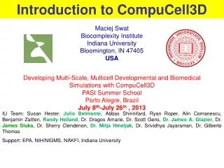
1. CompuCell3D Training Workshop Biocomplexity Institute Indiana University Bloomington, August 17-21 2009 Maciej Swat James Glazier Benjamin Zaitlen Randy Heiland Abbas Shirinifard

2. What you will learn during the workshop? • What is CompuCell3D? • Why use CompuCell3D? • Demo simulations • Glazier-Graner-Hogeweg (GGH) model – an overview • CompuCell3D architecture and terminology • XML 101. CC3DML-intro • Building first CompuCell3D simulation • Visualization package – CompuCell Player • Python scripting inside CompuCell3D • Building C++ CompuCell3D extension modules – for interested participants

3. What Is CompuCell3D? • CompuCell3D is a modeling environment used to build, test, run and visualize GGH-based simulations • CompuCell3D has built-in scripting language (Python) that allows users to quite easily write extension modules that are essential for building sophisticated biological models. • CompuCell3D thus is NOT a specialized software • Running CompuCell3D simulations DOES NOT require recompilation • CompuCell3D model is described using CompuCell3D XML and Python script(s) • CompuCell3D platform is distributed with a GUI front end – CompuCell Player. The Player provides 2- and 3-D visualization and simulation replay capabilities. • CompuCell3D is a cross platform application that runs on Linux/Unix, Windows, Mac OSX. CompuCell3D simulations can be easily shared

4. Why Use CompuCell3D? What Are the Alternatives? • CompuCell3D allows users to set up and run their simulations within minutes, maybe hours. A typical development of a specialized GGH code takes orders of magnitudes longer time. • CompuCell3D simulations DO NOT need to be recompiled. If you want to change parameters (in XML or Python scripts) or logic (in Python scripts) you just make the changes and re-run the simulation. With hand-compiled simulations there is much more to do. Recompilation of every simulation is also error prone and often limits users to those who have significant programming background. • CompuCell3D is actively developed , maintained and supported. On www.compucell3d.org website users can download manuals, tutorials and developer documentation. CompuCell3D has approx. 4 releases each year – some of which are bug-fix releases and some are major • CompuCell3D has many users around the world. This makes it easier to collaborate or exchange modules and results saving time spent on developing new model. • The Biocomplexity Institute organizes training workshops and mentorship programs. Those are great opportunities to visit Bloomington and learn biological modeling using CompuCell3D. For more info see www.compucell3d.org

5. Why model sharing and standards are important? • 99% of modeling done with custom written code is very hard/impossible to reproduce or verify. Even in best quality publications authors may forget to describe small details which are actually essential to reproduce the described work. • Using standard modeling tools instead of writing your own code improves chances of your research being reused or improved by other scientists. Note: in certain situations people might be interested in, precisely, the opposite. • When people spend most of their time working on new ideas rather than struggling to reproduce old results it greatly improves research efficiency • Bug tracking/bug bug detection is much more efficient with shared tools than with custom written ones. Bugs are also better documented for shared software. • Developing and sharing modules with other researchers is best way of improving software modeling tools used by community of researchers

6. Demo Simulations

7. The GGH Model – an Overview x 20 • Energy minimization formalism • - extended by Graner and Glazier, 1992 • DAH: Contact energy depending on cell types (differentiated cells) • Metropolis algorithm: probability of configuration change

8. Brief Explanation of Equation Symbols s(x) –denotes id of the cell occupying position x. All pixels pointed by arrow have same cell id , thus they belong to the same cell t(s(x)) denotes cell type of cell with id s(x). In the picture above blue and yellow cells have different cell types and different cell id. Arrows mark different cell types Notice that in your model you may (will) have many cells of the same type but with different id. For example in a simple cellsorting simulation there will be many cells of type “Condensing” and many cells with type “NonCondensinig”

9. CompuCell3D terminology • Spin-copy attempt is an event where program randomly picks a lattice site in an attempt to copy its spin to a neighboring lattice site. • Monte Carlo Step (MCS) consists of series spin-copy attempts. Usually the number of spin copy-attempts in single MCS is equal to the number of lattice sites, but this is can be customized • CompuCell3D Pluginis a software module that either calculates an energy term in a Hamiltonian or implements action in response to spin copy (lattice monitors). Note that not all spin-copy attempts will trigger lattice monitors to run. • Steppablesare CompuCell3D modules that are run every MCS after all spin-copy attempts for a given MCS have been exhausted. Most of Steppables are implemented in Python. Most customizations of CompuCell3D simulations is done through Steppables • Steppersare modules that are run for those spin-copy attempts that actually resulted in energy calculation. They are run regardless whether actual spin-copy occurred or not. For example cell mitosis is implemented in the form of stepper. • Fixed Steppers are modules that are run every spin-copy attempt.

10. CompuCell3D Terminology – Visual Guide Change pixel Spin copy “blue” pixel (newCell) replaces “yellow” pixel (oldCell) 100x100x1 square lattice = 10000 lattice sites (pixels) MCS 21 MCS 22 MCS 23 MCS 24 10000 spin-copy attempts 10000 spin-copy attempts 10000 spin-copy attempts 10000 spin-copy attempts Run Steppables Run Steppables Run Steppables

11. accept invalid attempt valid attempt valid attempt accept valid attempt valid attempt reject accept

12. Nearest neighbors in 2D and their Euclidian distances from the central pixel 3 5 4 4 5 4 1 2 2 4 1 3 1 3 1 2 4 4 2 3 4 4 5 5 Spin copy can take place between any order nearest neighbor (although in practice we limit ourselves to only few first oders). <NeighborOrder>2</NeighborOrder> 2nd nearest neighbor Contact energy calculation (see further slides) are also done up to certain order of nearest neighbors (default is 1) <NeighborOrder>2</NeighborOrder> Note: older tags still work but we encourage using new ones - they make more sense

13. 4 4 4 4 3 2 2 4 3 4 3 3 1 1 1 4 4 2 4 1 4 2 2 2 1 1 4 4 1 3 3 1 3 1 3 2 2 2 2 4 4 1 4 4 3 4 4 4 3 4 Nearest neighbors in 2D and their Euclidian distances from the central pixel

14. CompuCell3D Architecture Object oriented implementation in C++ and Python Visualization, Steering, User Interface Plugins Calculate change in energy Python Interpreter Biologo Code Generator Kernel Runs Metropolis Algorithm PDE Solvers Lattice monitoring

15. Typical “Run-Time” Architecture of CompuCell • CompuCell can be run in a variety of ways: • Through the Player with or without Python interpreter • As a Python script • As a stand alone computational kernel+plugins CompuCellPlayer Python CompuCell3D Kernel Plugins

16. XML 101 XML stands for eXtensible Markup Language. It is NOT a programming language. Its main purpose is to standarize information exchange between different applications. XML Example: <Sentence> <Text>It is too early to be in class</Text> <FontType>TimesNewRoman</FontType> <FontSize>12</FontSize> <DisplayHint Hint=“AddFrameAround”/> </Sentence>

17. CompuCell Related Example Defining basic properties of the simulation like lattice dimension, number of Monte Carlo Steps, Temperature and ratio of spin-copy attempts to number of lattice sites (Flip2DimRatio). <Potts> section has to be included in every CompuCell3D simulation <Potts> <Dimensionsx="71" y="36" z="211"/> <Steps>10</Steps> <Temperature>2</Temperature> <Flip2DimRatio>2</Flip2DimRatio> </Potts> Defining properties of Volume Energy term – cell target volume and lambda parameter: <PluginName=“Volume"> <TargetVolume>25</TargetVolume> <LambdaVolume>2.0</LambdaVolume> </Plugin> ...

18. Building Your First CompuCell3D Simulation Cell All simulation parameters are controlled by the config file. The config file allows you to only add those features needed for your current simulation, enabling better use of system resources. Define Lattice and Simulation Parameters < CompuCell3D> <Potts> <Dimensionsx=“100" y=“100" z=“1"/> <Steps>10</Steps> <Temperature>2</Temperature> <Flip2DimRatio>1</Flip2DimRatio> </Potts> … </CompuCell3D>

19. Cell Define Cell Types Used in the Simulation Each CompuCell3D xml file must list all cell types that will used in the simulation <Plugin Name="CellType"> <CellType TypeName="Medium" TypeId="0"/> <CellType TypeName=“Light" TypeId="1"/> <CellType TypeName=“Dark" ="2"/> </Plugin> Notice that Medium is listed with TypeId =0. This is both convention and a REQUIREMENT in CompuCell3D. Reassigning Medium to a different TypeId may give undefined results. This limitation will be fixed in one of the next CompuCell3D releases

20. Cell Define Energy Terms of the Hamiltonian and Their Parameters Volume volume volumeEnergy(cell) <Plugin Name="Volume"> <TargetVolume>25</TargetVolume> <LambdaVolume>1.0</LambdaVolume> </Plugin> <Plugin Name="Surface"> <TargetSurface>21</TargetSurface> <LambdaSurface>0.5</LambdaSurface> </Plugin> Surface area surfaceEnergy(cell) <Plugin Name="Contact"> <Energy Type1="Medium" Type2="Medium">0 </Energy> <Energy Type1="Light" Type2="Medium">16 </Energy> <Energy Type1="Dark" Type2="Medium">16 </Energy> <Energy Type1="Light" Type2="Light">16.0 </Energy> <Energy Type1="Dark" Type2="Dark">2.0 </Energy> <Energy Type1="Light" Type2="Dark">11.0 </Energy> </Plugin> Contact contactEnergy( cell1, cell2)

21. Plugin XML Syntax <Plugin Name="Volume"> <TargetVolume>25</TargetVolume> <LambdaVolume>1.0</LambdaVolume> </Plugin> <Plugin Name="Surface"> <TargetSurface>21</TargetSurface> <LambdaSurface>0.5</LambdaSurface> </Plugin>

22. Plugin XML Syntax – Contact Energy <Plugin Name="Contact"> <Energy Type1="Medium" Type2="Medium">0 </Energy> <Energy Type1="Light" Type2="Medium">16.0 </Energy> <Energy Type1="Dark" Type2="Medium">16.0 </Energy> <Energy Type1="Light" Type2="Light">16 </Energy> <Energy Type1="Dark" Type2="Dark">2.0 </Energy> <Energy Type1="Light" Type2="Dark">11.0 </Energy> </Plugin> 1-d term ensures that pixels belonging to the same cell do not contribute to contact energy

23. Laying Out Cells on the Lattice Using built-in cell field initializer: <Steppable Type="BlobInitializer"> <Region> <Radius>30</Radius> <Center x="40" y="40" z="0"/> <Gap>0</Gap> <Width>5</Width> <Types>Dark,Light</Types> </Region> </Steppable> This is just an example of cell field initializer. More general ways of cell field initialization will be discussed later. NOTE: In actual example Dark cells are called Condensingand Light cells NonCondensing

24. Putting It All Together - cellsort_2D.xml <CompuCell3D> <Potts> <Dimensions x="100" y="100" z="1"/> <Steps>10</Steps> <Temperature>2</Temperature> <Flip2DimRatio>1</Flip2DimRatio> </Potts> <Plugin Name="CellType"> <CellType TypeName="Medium" TypeId="0"/> <CellType TypeName=“Light" TypeId="1"/> <CellType TypeName=“Dark" ="2"/> </Plugin> <Plugin Name="Volume"> <TargetVolume>25</TargetVolume> <LambdaVolume>1.0</LambdaVolume> </Plugin> <Plugin Name="Surface"> <TargetSurface>21</TargetSurface> <LambdaSurface>0.5</LambdaSurface> </Plugin> <Plugin Name="Contact"> <Energy Type1="Medium" Type2="Medium">0 </Energy> <Energy Type1="Light" Type2="Medium">16 </Energy> <Energy Type1="Dark" Type2="Medium">16 </Energy> <Energy Type1="Light" Type2="Light">16 </Energy> <Energy Type1="Dark" Type2="Dark">2.0 </Energy> <Energy Type1="Light" Type2="Dark">11 </Energy> </Plugin> <Steppable Type="BlobInitializer"> <Region> <Radius>30</Radius> <Center x="40" y="40" z="0"/> <Gap>0</Gap> <Width>5</Width> <Types>Dark,Light</Types> </Region> </Steppable> </CompuCell3D> Coding the same simulation in C/C++/Java/Fortran would take you at least 1000 lines of code…

25. Putting It All Together - Avoiding Common Errors in XML code • First specify Potts section, then list all the plugins and finally list all the steppables. This is the correct order and if you mix e.g. plugins with steppables you will get an error. Remember the correct order is • Potts • Plugins • Steppables • 2. Remember to match every xml tag with a closing tag • <Plugin> • … • </Plugin> • 3. Watch for typos – if there is an error in the XML syntax CC3D will give you an error pointing to the location of an offending line • 4. Modify/reuse available examples rather than starting from scratch – saves a lot of time

26. Foam Coarsening simulation <CompuCell3D> <Potts> <Dimensions x="101" y="101" z="1"/> <Steps>1000</Steps> <Temperature>5</Temperature> <Flip2DimRatio>1.0</Flip2DimRatio> <Boundary_y>Periodic</Boundary_y> <Boundary_x>Periodic</Boundary_x> <NeighborOrder>2</NeighborOrder> </Potts> <Plugin Name="CellType"> <CellType TypeName="Medium" TypeId="0"/> <CellType TypeName="Foam" TypeId="1"/> </Plugin> <Plugin Name="Contact"> <Energy Type1="Foam" Type2="Foam">50</Energy> <NeighborOrder>2</NeighborOrder> </Plugin> <Steppable Type="PIFInitializer"> <PIFName>foaminit2D.pif</PIFName> </Steppable> </CompuCell3D>

27. CompuCellPlayer – the Best Way To Run Simulations Steering bar allows users to start or pause the simulation, zoom in , zoom out, to switch between 2D and 3D visualization, change view modes (cell field, pressure field , chemical concentration field, velocity field etc..) Player can output multiple views during single simulation run – Add Screenshot function Information bar

28. Opening a Simulation in the Player Go to File->Open Simulation File

29. Running Simulation From Command Line You can simply start the simulation with or without Player straight from command line Open up console (terminal) and type: ./compucell3d.command –i cellsort_2D.xml (on OSX) ./compucell3d.sh –i cellsort_2D.xml (on Linux) compucell3d.bat –i cellsort_2D.xml (on Windows) – or simply double click Desktop icon Running CompuCell3D from command line not only convenient, but sometimes (on clusters) the only option to run the simulation. For more information about command line options please see “Running CompuCell3D” manual available at www.compucell3d.org.

30. Running the Simulation • After typing the XML file in your favorite editor all you need to do to run the simulation is to open the XML file in the Player and hit “Play” button. • Screenshots from the simulations are automatically stored in the directory with name composed of simulation file name and a time at which simulation was started • As you can see, setting up CompuCell3D simulation was reasonably simple. • It is quite likely that if you were to code entire simulation in C/C++/Java etc. you would need much more time. • We hope that now you understand why using CompuCell3D saves you a lot of time and allows you to concentrate on biological modeling and not on writing low level computer code. • During last year we have improved CompuCell3D performance so that it is on par with hand-written code. Yet, if you really to have the fastest GGH code in the world you should write code your own simulation directly in C or even better in assembly language. Before you do it, make sure you want to spend time rewriting the code that already exist…

31. Choosing the Right Text Editor • Since developing CompuCell3D simulation requires typing some simple code it is important that you have the right tools to do that most effectively. • On Windows systems we highly recommend Notepad++ editor: • http://notepad-plus.sourceforge.net/uk/site.htm • On Linux you have lots of choices: Kate (my favorite), gedit, mcedit etc. • On OSX situation gets a bit complicated, but there is one editor called Smultron which is good for programming • http://sourceforge.net/projects/smultron/ • And as usual, if nothing else works there is always vi, and emacs

32. CompuCell Player 101

33. CompuCell Player – The Basics • Caution: CompuCellPlayer is still under development so some options may not work properly however, for the most part this is fully functional ComUCell3D front end and much better than its predecessor • For the most part , CompuCell Player is fairly intuitive to use. It is quite important to get familiar with configure options to the get most out of the Player • CompuCell Player is a graphical front-end to CompuCell3D computational part. It is written in Python using PyQt4 and VTK. It also uses C++ wrapped code for performance critical processing. • Because of PyQt4 , it provides native look and feel on Linux, OSX and Windows. This means that dialog and windows will look pretty much the same as other dialogs in your operating system. Traditionally, Qt tookits look the ugliest on OSX. • CompuCell Player provides basic visualization capabilities for CompuCell3D simulations. It automatically detects types of plots for given simulation. • Saves users the hassle of writing visualization code. • Helps debugging simulations • Next version of Player will allow users to write their own visualization pipeline using VTK standards

34. Capabilities of CompuCellPlayer– Why You Should Use the Player. • Provides wide range of visualization - cell field plots, concentration plots, vector field plots in both 2- and 3-D. • Allows to store multiple lattice views in a single run. For example users can store multiple projections of the cell lattice, concentration fields, various 3D views etc… in a single run. • Can be run in GUI and silent mode (i.e. without displaying GUI but still saving screenshots) • Is ready to be used on clusters that do not have X-server installed. This feature is essential for doing “production runs” of your simulations. • Concentration fields and vector fields initialized from Python level can easily be displayed in the Player. Yes, you can control the Player visualizations from Python level. • Configurable from XML level for those users who prefer typing to clicking

35. Configuring the Player Most of Player’s configuration options are accessible through Tools->Configuration… and Visualization menus.

36. Visualization Menu allows you to choose whether in 2D cell borders should be displayed or not (in 3D borders are not drawn at all). You can also select to draw isocontour lines for the concentration plots and turn on and off displaying of the information about minimum and maximum concentration.

37. Screen update frequency is a parameter that defines how often (in units of MCS) Player screen should be updated. Note, if you choose to update screen too often (say every MCS) you will notice simulation speed degradation because it does take some time to draw on the screen. You may also choose not to output any files by checking “Do not output results” check-box. Additionally you have the option to output simulation data in the VTK format for later replay. Screenshot frequency determines how often screenshots of the lattice views will be taken (currently Player outputs *.png files) .

38. Screenshots Screenshots are taken every “Screenshot Frequency” MCS By default Player will store screenshots of the currently displayed lattice view. In addition to this users can choose to store additional screenshots at the same time. Simply switch to different lattice view, click camera button. Those additional screenshots will be taken irrespectively of what Player currently displays. Once you selected additional screenshots it is convenient to save screenshot description file (it is written automatically by the Player, user just provide file name). Next time you decide to run CompuCell3D you may just use command compucell3d.sh -s screenshotDesctiptionFile_cellsort.txt -i cellsort_2D.xml This will run simulation where stored screenshots will be taken

39. Click camera button on select lattice views When you picked lattice views, you may save screenshot description file for later reuse Notice, you may change plot types as well

40. Configure->cell type colors… Enter cell type number here To enter new cell type click “Add Cell Type” button Click here to change color for cell type 1 Click here to change cell border color Click here to change isocontour color

41. Configure->Cell types invisible in 3D… Sometimes when you open up the simulation and switch to 3D view you may find that your simulation looks like solid a parallelepiped. This might be due to a box made out of frozen cells that hides inside other cells. In this case you need to make the box invisible. Type cell type number that you want to be invisible in 3D in this box. Notice, by default Player will not display Medium (type 0). Here we also make types 4 and 5 invisible

42. Steering the simulation CompuCell3D Player will allow you to change most of the parameters of the XML file while the simulation is running. Use steering panel to change simulation parameters. Make sure you pause simulation before doing this Target volume = 100 Screenshot was taken before simulation had time to equilibrate Target volume = 25

43. Using different kind of lattices with CompuCell3D • Current version of CompuCell3D allows users to run simulations on square and hexagonal lattices. • Other regular geometries (e.g. triangular) can be implemented fairly easily • Some plugins work on square lattice only - e.g. local connectivity plugin • Switching to hexagonal lattice requires only one line of code in the Potts section • <LatticeType>Hexagonal</LatticeType> • Model parameters may need to be adjusted when going from one type lattice to another. This is clearly an inconvenience but we will try to provide a solution in the future • Different lattices have varying degrees of lattice anisotropy. In many cases using lower anisotropy lattice is desired (e.g. foam coarsening simulation on hexagonal lattice). It is also important to check results of your simulation on different kind of lattices to make sure you don’t have any lattice-specific effects. • Compucell3D makes such comparisons particularly easy

44. 4 4 4 4 3 2 2 4 3 4 3 3 1 1 1 4 4 2 4 1 4 2 2 2 1 1 4 4 1 3 3 1 3 1 3 2 2 2 2 4 4 1 4 4 3 4 4 4 3 4 Nearest neighbors in 2D and their Euclidian distances from the central pixel SquareLattice: Square in 2D Cube in 3D Hexagonal lattice: Hexagon in 2D Rhombic dodecahedron in 3D

45. Cell-sorting simulation on square and hexagonal lattices The simulation parameters were kept the same for the two runs 1000 MCS 1000 MCS

46. Cell Attributes CompuCell3D cells have a default set of attributes: Volume, surface, center of mass position, cell id etc… Additional attributes are added during runtime: List of cells neighbors, polarization vector etc… To keep parameters up-to-date users need to declare appropriate plugins in the CC3DML configuration file. For example, to make sure surface of cell is up-to-date users need to make sure that SurfaceTracker plugin is registered: Include : <Plugin Name=“SurfaceTracker”/>

47. or use Surface plugin which will implicitly call SurfaceTracker <Plugin Name=“Surface”> <LambdaSurface>0.0</LambdaSurface> <TargetSurface>25.0</TargetSurface> </Plugin> But here surface tracking costs you extra calculation of surface energy term: E=…+l(s-ST)2 +…

48. More Flexible Specification of Surface and Volume Constraints <Plugin Name="VolumeFlex"> <VolumeEnergyParameters CellType=“Amoeba" TargetVolume=“150" LambdaVolume="10"/> <VolumeEnergyParameters CellType=“Bacteria" TargetVolume=“10" LambdaVolume=“50"/> </Plugin> You may specify different volume and surface constraints for different cell types. This can be done entirely at the XML level. Type dependent quantities <Plugin Name=“SurfaceFlex"> <SurfaceEnergyParameters CellType=“Amoeba" TargetSurface=“60" LambdaSurface="10"/> <SurfaceEnergyParameters CellType=“Bacteria" TargetSurface=“12" LambdaSurface=“20"/> </Plugin>

49. Even More Flexible Specification of Surface and Volume Constraints <Plugin Name="VolumeLocalFlex“/> <Plugin Name=“SurfaceLocalFlex“/> Notice that all the parameters are local to a cell. Each cell might have different target volume (target surface) and different l volume (surface). You will need to use Python to initialize or manipulate those parameters while simulation is running. There is currently no way to do it from XML level. I am not sure it would be practical either.

50. Tracking Cell Neighbors Sometimes in your simulation you need to have access to a current list of cell neighbor. CompuCell3D makes this task easy: <Plugin Name=“NeighborTracker“/> Inserting this statement in the plugins section of the XML will ensure that at any given time the list of cell neighbors will be accessible to the user. You can access such a list either using C++ or Python. In addition to storing neighbor list , a common surface area of a cell with its neighbors is stored.