Aperture Photometry with CCD Images using IRAF
350 likes | 631 Vues
Aperture Photometry with CCD Images using IRAF . Kevin Krisciunas. Images must be taken in a sensible manner. Ask advice from experienced observers. But remember Wallerstein’s Rule: “Four astronomers, five opinions.” Some people prefer dome flats.

Aperture Photometry with CCD Images using IRAF
E N D
Presentation Transcript
Aperture Photometry with CCD Images using IRAF Kevin Krisciunas
Images must be taken in a sensible manner. Ask advice • from experienced observers. But remember Wallerstein’s • Rule: “Four astronomers, five opinions.” • Some people prefer dome flats. • I prefer sky flats (pointless if there are visible clouds). • After focusing camera at start, do one standards • field in all the filters you will use. • Finish the night with a standards field. • Do standards every 90 minutes or so. It is the only • way to prove that the night was photometric. The • CCD detector is a much better cloud detector than • your eyes…
If your program objects are observed low in the sky and high in the sky, you better observe standards low in the sky and high in the sky so that you can measure the effect of the atmosphere. If your program stars are very red or very blue, you better observe standard stars that are even redder or bluer, so that you can interpolate transformations rather than extrapolate them. Or you may realize that you need non-linear transformations.
Popular lists of standards: UBVRI – Landolt (1992), Landolt (2007) Sloan filters – J. Allyn Smith et al. (2002) Most field stars are red. Many Landolt fields have one very blue star like Rubin 149 and a number of redder stars, allowing you to determine photometric color terms easily.
For crowded fields you have to reduce your photometry with DAOPHOT or DOPHOT. This involves determining the point spread function of the instrument. The PSF can vary with position in a frame or from frame to frame. Plots made with IRAF task “imexam” with options r (for radial plot) or s (for surface plot).
If you have non-crowded fields, aperture photometry can often be much more straightforward. And there are some advantages: If the focus slowly degrades over the course of the night or you have slight tracking errors (giving stellar images that are not round), with a software aperture of radius 8 or 10 pixels, you can still put more than 98 percent of the light into that aperture. 8 px might be OK for observations high in the sky, but seeing is worse for observations low in the sky. The underlying sky level is determined by using an annulus (say from radius 12 to 20 pixels) centered on each star. IRAF allows you to easily get around faint stars or cosmic ray hits in the sky annulus.
Say you observe with UBVRI filters. The goal is to convert the instrumental magnitudes of the standards to a photometric system such as Landolt’s. One assumes that the CCD detector is linear, namely that the arrival of twice as many photons produces twice as many countable electrons. Some cameras are demonstrably non-linear at high count rates, such as the Las Campanas 1-m camera. In that case the observer has to make sure that one doesn’t exceed the recommended count limit on the stars of interest, or one must correct for this after the fact (which would be a hassle).
We transform the instrumental magnitudes of the standards to some photometric system using linear equations such as: U = u – kuX + CTu(u-b) + zpu B = b – kbX + CTb(b-v) + zpb V = v – kvX + CTv(b-v) + zpv R = r – krX + CTr(v-r) + zpr I = i – kiX + CTi(v-i) + zpi UBVRI are “catalog magnitudes” from Landolt. ubvri are instrumental magnitudes from IRAF. k’s are extintinction coefficients for the atmosphere. X = “air mass”. CT’s are “color terms”. zp’s are photometric zeropoints.
The “air mass” X is the path length through the atmosphere toward the field you are observing, compared to the path length through the atmosphere toward the zenith. Most observing is done more than 30 degrees above the horizon (zenith angle 60 degrees). We can use a plane atmosphere approximation and take X = secant of the zenith angle. So – it is determined from spherical trigonometry. Typical extinction coefficients at Cerro Tololo are ku = 0.51, kb = 0.26, kv = 0.15, kr = 0.11, and ki = 0.06 magnitudes per air mass. But – these can vary +/- 20 % from clear night to clear night. The U-band coefficient might vary 20 percent over the course of a single night.
If you have a night’s worth of images taken in a sensible fashion and they are properly flat fielded, IRAF will allow you to determine the extinction coefficients, color terms, and zero points. Then, observations of stars and supernovae of unknown brightness, made with the same telescope and camera on that night, can be transformed to the same photometric system.
It helps to have a hardcopy of a log of the images for a particular night. Of course it is sensible to put the images for each night into separate subdirectories. Know your FITS header parameters of interest, for example Universal Time, object name, filter, exposure time, and airmass. The parameter names vary from observatory to observatory. You can double check an image whatever.fits by doing something like this: > imhead whatever l+ | page Then you might make a log file doing this: > hselect *.fits $I,ut,object,filter2,exptime,airmass yes > something.log
epar datapars • To set valid data range, read noise, gain (number of electrons • per ADU), and names of key FITS header parameters.
epar fitskypars • To set the sky fitting algorithm (“median” or “mode” better • than “mean”) and the sky annulus parameters. Exiting an option list is done via “:q”
epar photpars • To specify the list of aperture radii in pixels. You can • decide later which aperture is best for the night in • question. Now we’re ready to obtain some aperture magnitudes with IRAF’s apphot task “phot”. You put the little circle on a star in your SAOimage (ds9) window and hit the space bar.
This lists the image name, the pixel coordinates of the stars, and starting in column 5 the instrumental aperture magnitudes for radius = 6, 7, 8, 9, and 10 pixels.
Say a particular field was imaged in the U, B, V, R, and I filters, producing a set of files obj216.fits through obj220.fits. The telescope tracking might have drifted a little over time. A file of the pixel shifts between the images might contain these five lines for this set of images: obj216 0 0 obj217 -3 5 obj218 -4 7 obj219 -6 9 obj220 -8 11 I put all the sets of shifts on a given night into one file, called something like nov26.shifts
Next one exits “apphot” and invokes “photcal” in IRAF. One can create a text file of the U, B, V, R, I aperture photometry on a given field using “mknobsfile”. Parameters are set via “epar mknobsfile” then executing the action with “:go” We will also be using “fitparams” and “evalfit”.
File ru149.imsets might contain only one line: ru149 : obj216 obj217 obj218 obj219 obj220 We decided to use the 5th aperture specified by “photpars” (radius = 10 px).
Having generated a number of text files with “mknobsfile” containing the aperture magnitudes for each star in each filter, one uses an editor and creates a single file such as stds.raw . Then one can solve for the coefficients for all the photometric transformations using program “fitparams”.
File ubvri is derived from Landolt (1992, 2007) or some other list of magnitudes and/or colors. Here the variable BV is the B-V color, UB is the U-B color, etc. IRAF insists that the names of your standards in your raw data file match the ID’s in your catalog file.
Beginning and end of the file ubvri_ext.config which is used to specify the transforma- tion to the standard photometric system. One can give default starting values for certain parameters. Here, for example, V+BV means V mag from ubvri + B-V color, which equals B magnitude.
We should point out that if all the observations were taken at just about the elevation angle, there is very little range of air mass for the observations. In that case one should just adopt sensible mean values of extinction for the site and use simpler transformation equations, solving only for zeropoints and color terms.
Example of B-band fit for Nov 26, 2005, photometry with CTIO 0.9-m telescope. RMS error +/- 0.018 mag zpb = -2.887 +/- 0.011 kb = 0.279 +/- 0.007 mag/airmass CTb = -0.102 +/- 0.004 (part of file nov26.out)
On this night we obtained the following. This is about as good as it gets doing ground based photometry. Filter RMS extinction U +/- 0.044 0.504 (0.032) B 0.018 0.279 (0.007) V 0.016 0.160 (0.006) R 0.012 0.121 (0.004) I 0.021 0.072 (0.008)
Using stds.raw, ubvri_ext.config, and your catalog file of magnitudes and colors of standards (ubvri) you can use program “evalfit” to apply the derived transformations to all the observations of the standards. The output file gives the differences between your UBVRI magnitudes and those of Landolt. If your residuals change steadily from -0.05 to +0.05 over the course of the night, that indicates the photometric zeropoint was slowly changing over the night. A truly photometric night should show random small pluses and minuses in these residuals vs. time.
Portion of file stds.calib (output of task “evalfit”). Starting in column 4, every 3rd column gives “catalog value minus our value”.
Finally … • Obtain the aperture magnitudes for all your • research stars for all the frames and filters using “phot”. • Use “mknobsfile” to create files such as ngc1234.raw • (you have to use the same aperture size as for standards) • Use files such as ubvri_ext.config, nov26.out and • IRAF program “evalfit” to apply transformations to • convert instrumental magnitudes on research objects • to standardized photometric system.