Download
1 / 66
850 likes | 1.48k Vues
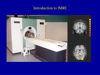
1. Introduction to fMRI. 2. Basic fMRI Physics. 3. Data Analysis. 4. Localisation. 5. Cortical Anatomy. 1. Introduction to fMRI. MRI vs. fMRI. Functional MRI (fMRI) studies brain function. MRI studies brain anatomy. Brain Imaging: Anatomy. Brain Imaging: Anatomy. CAT. PET.

E N D
1. Introduction to fMRI 2. Basic fMRI Physics 3. Data Analysis 4. Localisation 5. Cortical Anatomy
MRI vs. fMRI Functional MRI (fMRI) studies brain function. MRI studies brain anatomy.
Brain Imaging: Anatomy Brain Imaging: Anatomy CAT PET Photography MRI Source: modified from Posner & Raichle, Images of Mind
MRI vs. fMRI MRI fMRI high resolution (1 mm) low resolution (~3 mm but can be better) one image • fMRI • Blood Oxygenation Level Dependent (BOLD) signal • indirect measure of neural activity: active neurons shed oxygen and become more magnetic increasing the fMRI signal many images (e.g., every 2 sec for 5 mins) neural activity blood oxygen fMRI signal
Brain Activity Time fMRI Activation Flickering Checkerboard OFF (60 s) - ON (60 s) -OFF (60 s) - ON (60 s) - OFF (60 s) Source: Kwong et al., 1992
PET and fMRI Activation Source: Posner & Raichle, Images of Mind
fMRI Experiment Stages: Prep • 1) Prepare subject • Consent form • Safety screening • Instructions • 2) Shimming • putting body in magnetic field makes it non-uniform • adjust 3 orthogonal weak magnets to make magnetic field as homogenous as possible • 3) Sagittals • Take images along the midline to use to plan slices Note: That’s one g, two t’s
fMRI Experiment Stages: Anatomicals • 4) Take anatomical (T1) images • high-resolution images (e.g., 1x1x2.5 mm) • 3D data: 3 spatial dimensions, sampled at one point in time • 64 anatomical slices takes ~5 minutes
VOXEL (Volumetric Pixel) Slice Thickness e.g., 6 mm In-plane resolution e.g., 192 mm / 64 = 3 mm 3 mm 6 mm SAGITTAL SLICE IN-PLANE SLICE 3 mm Number of Slices e.g., 10 Matrix Size e.g., 64 x 64 Field of View (FOV) e.g., 19.2 cm Slice Terminology
first volume (2 sec to acquire) fMRI Experiment Stages: Functionals • 5) Take functional (T2*) images • images are indirectly related to neural activity • usually low resolution images (3x3x5 mm) • all slices at one time = a volume (sometimes also called an image) • sample many volumes (time points) (e.g., 1 volume every 2 seconds for 150 volumes = 300 sec = 5 minutes) • 4D data: 3 spatial, 1 temporal …
ROI Time Course fMRI Signal (% change) ~2s Condition Time Condition 1 Statistical Map superimposed on anatomical MRI image Condition 2 ... Region of interest (ROI) ~ 5 min Functional images Activation Statistics Time
Use stat maps to pick regions Then extract the time course Statistical Maps & Time Courses
condition: one set of stimuli or one task 4 stimulus conditions + 1 baseline condition (fixation) Design Jargon: Runs session: all of the scans collected from one subject in one day run (or scan): one continuous period of fMRI scanning (~5-7 min) experiment: a set of conditions you want to compare to each other Note: Terminology can vary from one fMRI site to another (e.g., some places use “scan” to refer to what we’ve called a volume). A session consists of one or more experiments. Each experiment consists of several (e.g., 1-8) runs More runs/expt are needed when signal:noise is low or the effect is weak. Thus each session consists of numerous (e.g., 5-20) runs (e.g., 0.5 – 3 hours)
run epoch: one instance of a condition first “objects right” epoch second “objects right” epoch volume #1 (time = 0) volume #105 (time = 105 vol x 2 sec/vol = 210 sec = 3:30) epoch 8 vol x 2 sec/vol = 16 sec Time Design Jargon: Paradigm paradigm (or protocol): the set of conditions and their order used in a particular run
Recipe for MRI • 1) Put subject in big magnetic field (leave him there) • 2) Transmit radio waves into subject [about 3 ms] • 3) Turn off radio wave transmitter • 4) Receive radio waves re-transmitted by subject • Manipulate re-transmission with magnetic fields during this readout interval [10-100 ms: MRI is not a snapshot] • 5) Store measured radio wave data vs. time • Now go back to 2) to get some more data • 6) Process raw data to reconstruct images • 7) Allow subject to leave scanner (this is optional) Source: Robert Cox’s web slides
most likely explanation: nuclear has bad connotations less likely but more amusing explanation: subjects got nervous when fast-talking doctors suggested an NMR History of NMR • NMR = nuclear magnetic resonance • Felix Block and Edward Purcell • 1946: atomic nuclei absorb and re-emit radio frequency energy • 1952: Nobel prize in physics • nuclear: properties of nuclei of atoms • magnetic: magnetic field required • resonance: interaction between magnetic field and radio frequency Bloch Purcell NMR MRI: Why the name change?
History of fMRI MRI -1971: MRI Tumor detection (Damadian) -1973: Lauterbur suggests NMR could be used to form images -1977: clinical MRI scanner patented -1977: Mansfield proposes echo-planar imaging (EPI) to acquire images faster fMRI -1990: Ogawa observes BOLD effect with T2* blood vessels became more visible as blood oxygen decreased -1991: Belliveau observes first functional images using a contrast agent -1992: Ogawa et al. and Kwong et al. publish first functional images using BOLD signal Ogawa
Necessary Equipment 4T magnet RF Coil gradient coil (inside) Magnet Gradient Coil RF Coil Source: Joe Gati, photos
1 Tesla (T) = 10,000 Gauss • Earth’s magnetic field = 0.5 Gauss • 4 Tesla = 4 x 10,000 0.5 = 80,000X Earth’s magnetic field Main field = B0 Robarts Research Institute 4T B0 x 80,000 = Source: www.spacedaily.com The Big Magnet Very strong Continuously on
Magnet Safety The whopping strength of the magnet makes safety essential. Things fly – Even big things! Source: www.howstuffworks.com Screen subjects carefully Make sure you and all your students & staff are aware of hazzards Develop stratetgies for screening yourself every time you enter the magnet Source: http://www.simplyphysics.com/ flying_objects.html
Subject Safety • Anyone going near the magnet – subjects, staff and visitors – must be thoroughly screened: • Subjects must have no metal in their bodies: • pacemaker • aneurysm clips • metal implants (e.g., cochlear implants) • interuterine devices (IUDs) • some dental work (fillings okay) • Subjects must remove metal from their bodies • jewellery, watch, piercings • coins, etc. • wallet • any metal that may distort the field (e.g., underwire bra) • Subjects must be given ear plugs (acoustic noise can reach 120 dB) This subject was wearing a hair band with a ~2 mm copper clamp. Left: with hair band. Right: without. Source: Jorge Jovicich
Outside magnetic field Protons align with field • randomly oriented Inside magnetic field • spins tend to align parallel or anti-parallel to B0 • net magnetization (M) along B0 • spins precess with random phase • no net magnetization in transverse plane • only 0.0003% of protons/T align with field M longitudinal axis Longitudinal magnetization transverse plane Source: Mark Cohen’s web slides M = 0 Source: Robert Cox’s web slides
fMRI Basics – The functional magnetic resonance imaging technique measures the amount of oxygen in the blood in small regions of the brain. These regions are called voxels. Neural activity uses up oxygen and the vasculature responds by providing more highly oxygenated blood to local brain regions. Thus a change in amount of oxygen in the blood is measured, and this is taken as a proxy for the amount of local neural activity. The measured signal is often called the BOLD signal (Blood Oxygen Level Dependent). Because neural activity is not measured directly, one needs to think about what the indirect signal really tells us, and how it’s spatial and temporal resolution are limited. Certainly, however,the BOLD signal tells us something about localization of neural activity in the brain.
BOLD signal Blood Oxygen Level Dependent signal • neural activity blood flow oxyhemoglobin T2* MR signal Mxy Signal Mo sin T2* task T2* control Stask S Scontrol time TEoptimum Source: fMRIB Brief Introduction to fMRI Source: Jorge Jovicich
BOLD signal Source: Doug Noll’s primer
Hypotheses vs. Data • Hypothesis-driven • Examples: t-tests, correlations, general linear model (GLM) • a priori model of activation is suggested • data is checked to see how closely it matches components of the model • most commonly used approach • Data-driven • Independent Component Analysis (ICA) • no prior hypotheses are necessary • multivariate techniques determine the patterns in the data that account for the most variance across all voxels • can be used to validate a model (see if the math comes up with the components you would’ve predicted) • can be inspected to see if there are things happening in your data that you didn’t predict • can be used to identify confounds (e.g., head motion) • need a way to organize the many possible components • new and upcoming
Comparing the two approaches • Region of Interest (ROI) Analyses • Gives you more statistical power because you do not have to correct for the number of comparisons • Hypothesis-driven • ROI is not smeared due to intersubject averaging • Easy to analyze and interpret • Neglects other areas which may play a fundamental role • Popular in North America • Whole Brain Analysis • Requires no prior hypotheses about areas involved • Includes entire brain • Can lose spatial resolution with intersubject averaging • Can produce meaningless “laundry lists of areas” that are difficult to interpret • Depends highly on statistics and threshold selected • Popular in Europe NOTE: Though different experimenters tend to prefer one method over the other, they are NOT mutually exclusive. You can check ROIs you predicted and then check the data for other areas. Source: Tootell et al., 1995
Why do we need statistics? • MR Signal intensities are arbitrary • -vary from magnet to magnet, coil to coil, within a coil (especially surface coil), day to day, even run to run • -may also vary from area to area (some areas may be more metabolically active) • We must always have a comparison condition within the same run We need to know whether the “eyeball tests of significance” are real. Because we do so many comparisons, we need a way to compensate.
Localize “motion area” MT in a run comparing moving vs. stationary rings Extract time courses from MT in subsequent runs while subjects see illusory motion (motion aftereffect) MT • A. ROI approach • Do (a) localizer run(s) to find a region (e.g., show moving rings to find MT) • Extract time course information from that region in separate independent runs • See if the trends in that region are statistically significant • Because the runs that are used to generate the area are independent from those used to test the hypothesis, liberal statistics can be used Two approaches: ROI Example study: Tootell et al, 1995, Motion Aftereffect Source: Tootell et al., 1995
BRAIN LOCALIZATION AND ANATOMYwith an emphasis on cortical areas • Why so corticocentric? • cortex forms the bulk of the brain • subcortical structures are hard to image (more vulnerable to motion artifacts) and resolve with fMRI • cortex is relevant to many cognitive processes • neuroanatomy texts typically devote very little information to cortex • Caveats of corticocentrism: • other structures like the cerebellum are undoubtedly very important (contrary to popular belief it not only helps you “walk and chew gum at the same time” but also has many cognitive functions) but unfortunately are poorly understood as yet • need to remember there may be lots of subcortical regions we’re neglecting
How can we define regions? • Talairach coordinates • Anatomical localization • Functional localization • Region of interest (ROI) analyses
Talairach & Tournoux, 1988 • squish or stretch brain into “shoe box” • extract 3D coordinate (x, y, z) for each activation focus Talairach Coordinate System Individual brains are different shapes and sizes… How can we compare or average brains? Note: That’s TalAIRach, not TAILarach! Source: Brain Voyager course slides
Corpus Callosum Fornix Pineal Body “bent asparagus” Rotate brain into ACPC plane Find anterior commisure (AC) Find posterior commisure (PC) ACPC line = horizontal axis Note: official Tal sez use top of AC and bottom of PC Source: Duvernoy, 1999
Squish or stretch brain to fit in “shoebox” of Tal system z y<0 AC=0 y>0 y y>0 ACPC=0 y<0 x Deform brain into Talairach space • Mark 8 points in the brain: • anterior commisure • posterior commisure • front • back • top • bottom (of temporal lobe) • left • right Extract 3 coordinates
Neurologic (i.e. sensible) convention • left is left, right is right L R - + x = 0 • Radiologic (i.e. stupid) convention • left is right, right is left R L + - x = 0 Left is what?!!! Note: Make sure you know what your magnet and software are doing before publishing left/right info! Note: If you’re really unsure which side is which, tape a vitamin E capsule to the one side of the subject’s head. It will show up on the anatomical image.
How to Talairach • For each subject: • Rotate the brain to the ACPC Plane (anatomical) • Deform the brain into the shoebox (anatomical) • Perform the same transformations on the functional data • For the group: • Either • Average all of the functionals together and perform stats on that • Perform the stats on all of the data (GLM) and superimpose the statmaps on an averaged anatomical (or for SPM, a reference brain) Averaged anatomical for 6 subjects Averaged functional for 7 subjects
Brodmann’s Areas Brodmann (1905): Based on cytoarchitectonics: study of differences in cortical layers between areas Most common delineation of cortical areas More recent schemes subdivide Brodmann’s areas into many smaller regions Monkey and human Brodmann’s areas not necessarily homologous
Talairach Pros and Cons • Advantages • widespread system • allows averaging of fMRI data between subjects • allows researchers to compare activation foci • easy to use • Disadvantages • based on the squished brain of an elderly alcoholic woman (how representative is that?!) • not appropriate for all brains (e.g., Japanese brains don’t fit well) • activation foci can vary considerably – other landmarks like sulci may be more reliable
gray matter (dendrites & synapses) GYRUS white matter (axons) SULCUS BANK FUNDUS Anatomical LocalizationSulci and Gyri pial surface gray/white border SULCUS FISSURE GYRUS Source: Ludwig & Klingler, 1956 in Tamraz & Comair, 2000
Variability of Sulci Variability of Sulci Source: Szikla et al., 1977 in Tamraz & Comair, 2000
Variability of Functional Areas Watson et al., 1995 -functional areas (e.g., MT) vary between subjects in their Talairach locations -the location relative to sulci is more consistent Source: Watson et al. 1995
Cortical Surfaces segment gray-white matter boundary render cortical surface inflate cortical surface sulci = concave = dark gray gyri = convex = light gray • Advantages • surfaces are topologically more accurate • alignment across sessions and experiments allows task comparisons Source: Jody Culham
Cortical Inflation Movie Movie: unfoldorig.mpeg http://cogsci.ucsd.edu/~sereno/unfoldorig.mpg Source: Marty Sereno’s web page