Production Economics
1.08k likes | 2.83k Vues
Production Economics. Introduction. Basic input-output relationships: How do we allocate finite resources? Aquaculture production changes as new technologies appear New varieties of inputs as well as combinations thereof Nothing is produced with one input!. Production Economics.

Production Economics
E N D
Presentation Transcript
Introduction • Basic input-output relationships: How do we allocate finite resources? • Aquaculture production changes as new technologies appear • New varieties of inputs as well as combinations thereof • Nothing is produced with one input!
Production Economics • Production economics: applying microeconomics to aquaculture • Studying production principles should clarify, for the farmer, issues such as costs, output response to input and the use of resources to maximize profit/minimize costs • REM: production economics is multi-disciplinary • Must look beyond the biology of production
Production Economics: Questions to be Answered • What is efficient production? • How is the most profitable amount of input determined? • How will farm production respond to a change in the price of an output (fish price)? • What enterprise combinations will maximize farm profits? • How much should farmers pay for a “pump”? • How will technical change affect output?
Production Economics: complexity • Crops grow in seasonal cycles and are affected by many inputs • some inputs are controlled by the manager, others are outside control (e.g., weather) • these are random events • time is also important (redfish production cycle vs. shrimp) • How do economists deal with these differences?
Economics and Production Complexity • Aquaculturists can vary rates of fertilizer, stocking densities, feed, feed ingredient level, aeration, etc. in ponds • Response is evaluated in terms of yield • economists do the same, but with data generated from previous production cycles, runs, etc. • Difference: aquaculture research and production lives in the “here and now”, economists are not “experimental” and use only existing data • They don’t try to control the inputs. Example: they have no control over prices, but simply look at what price was in effect when a previous production cycle occurred • Bottom line: they manipulate nothing, dependent variable response already known
Production Theory: Classification of Inputs • Those controlled by the manager: variable inputs • examples: rate of fertilization, feed rate • fixed inputs: those that don’t change for the production cycle or length of trial • examples: harvesting pump; feed silos, vehicles, land • random inputs: associated with nature or economics beyond that of the farm • remember: growing seasons are unique
Production Theory: assumptions that make it work • Some factors don’t change: continuous for entire production cycle (e.g., level of technology, land ownership, govt. programs) • production curve is smooth, well-behaved (e.g., fertilizer, labor is bad ex.) • perfect certainty: mgr has perfect insight • no time discounting* of production (removes time element from consideration) • manager is motivated by profits and is rationally seeking to optimize them *Basically, it means that a desired result in the future is perceived as less valuable than one in the present. For example, if you allow people to choose from being paid an amount in one year as opposed to being paid a smaller amount now, they will settle for a much smaller payment right now than they will in the future.
Production Theory Assumptions • Purpose of assumptions is not to deny the existence of real-world forces on production • purpose is to simplify the analysis to a point where a reasonable starting point can be identified • example: fish farmer deciding, after first experiment, to work with a wider stocking density, over more years • after the elementary theory has been developed, each additional source of complexity can be evaluated
Goals of Production Economics • assist farm managers in determining the best use of resources, given changing needs, values and goals of society • assist policy makers in determining the consequences of alternative public policies on output, profits, and use of resources on the farm • evaluate the uses of the theory of the firm for improving farm management and understanding the behavior of the farm as a profit-maximizing entity
Goals of Production Economics (continued) • evaluate the effects of technical and institutional changes on aquaculture production and resource use • determine individual farm and aggregated regional farm adjustments to output supply and resource use to changes in economic variables in the economy
How it works: • The effect of a single input on output can be determined if only that input is varied and all others are held constant. • Involves: • concept of the production function • average and marginal physical product • various stages of production
Concept of a Production Function • The production function represents an input-output relationship • describes the rate at which resources are transformed into products • relationships vary: animal variety, soil types, water quality, technologies, El Niño • any given input-output relationship specifies the quantities and qualities of resources needed to produce a particular product
The Production Function • The function can be expressed in many ways: • written form:Y = f(X1, X2, X3,…, Xn) • Y = output or yield • X’s are different inputs that take part in the production of Y • examples: yield is a function of stocking density, feed rate • Note: this written equation/form does not specify the importance or contribution of inputs to the production process
The Production Function • The production function can also be shown in either tabular or graphical form • Usually picks one variable input and studies the effect on yield • “Yield” is also referred to as total physical product or TPP • Keeps all other variable inputs “fixed” as well as traditional fixed inputs • let’s look at an example
Empirical Example FertilizerYield 0 lbs/ha 0 lbs 20 37 40 139 60 288 80 469 100 667 120 864 140 1045 160 1195 180 1296 200 1333 220 1291 TPP curve Tabular form Graphical form
Empirical Example • Data in the previous table/figure represent a production function relating shrimp yields to applied fertilizer • units of fertilizer (e.g., nitrogen and phosphate) represent the variable input, while all other inputs needed to produce shrimp (seed, labor, fuel, land) are the fixed inputs • But hey, I thought fuel, seed, etc. were variable inputs! Typically, yes, but in this case they remain constant • As shown, large increases in yield result from initial fertilizer applications
Empirical Example • However, yield increases become smaller at higher levels of application • A max of 1,330 lbs/ha was achieved with 200 lbs of fertilizer, afterwards declining • Zero yield with zero input, in reality, is uncommon in aquaculture; however, due to infertility of incoming water, soil, etc. • Note: Although farmers don’t typically use these functions, as such, they have mental pictures of what would happen, based on experience
More detail on the Classical Production Function Other characteristics of production function curves: • the production function is a continuous curve • inputs and outputs are perfectly divisible (otherwise, it would look like a series of dots) • inputs and outputs are homogenous (prices of product at one level of input are similar to others) Total physical product (TPP) Curve
Production Assumptions (1) Perfect Certainty • To use the production function, economists, farmers, etc. must agree upon the outcome (yield) for each unit of input • past results (e.g. shrimp yields in response to fertilizer) must at least approximate this year’s function (perfect certainty again…) • thus, the production function is a planning device
Perfect Certainty • Knowing how inputs will perform is difficult year to year in new industries such as aquaculture • It helps if you are reasonably sure and on top of results (literature, market evaluations, coffee shop…) • This is one of the big differences between standard agriculture and aquaculture • In aquaculture, no two sites are the same – inputs often function differently from one site to the next • Reality: care must be given to select the appropriate production function
Production Assumption 2: level of technology • If you produce, it is assumed that you do it via a certain methodology or process: which method? • However, we normally assume in production economics that the manager uses the most up-to-date technology • Translation: we assume the farmer uses the process that yields the most output from a given amount of input
Production Assumption 3: length of time period • The production function shows output at various levels of input over a specific length of time • As a result, all inputs (except the one you’re evaluating ) are fixed • reasons for fixing a variable • maybe the amount used is just the right amount, any more or less would lower profits • maybe the production time period is too short to change the amount of resource on hand (e.g., land) • the farmer just may not want to change the amount of resource (e.g., not changing the number of dairy cattle in order to evaluate a feed effect)
How to Work with the Production Function • There are several classical production functions for various agricultural situations • Problem: few are reported for aquaculture • The following are general guidelines and indications useful to farm managers
Three Stages of Production • First Stage: the average rate at which variable input (X) is transformed into product (Y) increases until it reaches its maximum (i.e., Y/X is at its maximum) • this maximum indicates the end of Stage 1
Production Stage 1 • Stage 1 deals with increasing production efficiency • Production efficiency is not always the maximum production level!! • This efficiency is known as average physical product, APP and is determined by dividing yield by its corresponding amount of input (Y/X) • Stage 1 ends where Y/X is largest, around 150 lbs input
Three Stages of Production • Stage 2: physical efficiency of the variable input is at a peak at the beginning of Stage 2 • Stage 2 ends when yield (APP) is at its maximum • Bottom line: maximum efficiciency does not equal maximum production I II III APP curve TPP curve
I II III APP curve TPP curve
Three Stages of Production • Stage 3: starts once TPP starts to decline • result of excessive quantities of variable input combined with fixed inputs • in order for all this to make sense, we need to understand that production functions are used to determine the most profitable amount of variable input and output • the production function allows you to make recommendations about input use even when input/output prices are unknown
What this Describes: Law of Diminishing Returns • Originally developed by early economists to describe the relationship between output and a variable input, when other inputs are constant • if increasing the amount of one input is added to a production process while all others are constant, additional output will eventually decrease • implies there is a “right” level of variable input to use with the combination of fixed inputs
Law of Diminishing Returns • Requires that the method of production does not change as variable input changes • does not apply when all inputs are varied • when theLDRis applied to production you get the classical production function • increasing marginal returns at first and decreasing marginal returns afterwards • it is possible that marginal returns could decrease in the beginning with the first application of the variable input
Economic Recommendations • 1) using logic you can see that if your production follows that of the example given, you should increase inputs to achieve a production level at least until Stage 2 is reached; • it doesn’t make sense to stop increasing input if its efficiency is increasing • 2) even if inputs are free, you don’t want to be in Stage 3; • the largest amount of input you would use is that at the end of Stage 2 • the area of economic relevance is within Stage 2 for firms that buy and sell in competitive markets • fine tuning comes from knowing prices
Homework 4: due next time 1) Develop a production curve using the following data: Stocking (fry/ac) Harvest Biomass (lb/ac) 0 0 1,000 185 2,000 695 3,000 1,440 4,000 2,345 5,000 3,335 6,000 4,320 7,000 5,225 8,000 5,975 9,000 6,480 10,000 6,665 11,000 6455 2) At what level of input would Stage 2 start?