Download
1 / 13
130 likes | 931 Vues
Fugacity of Non-Ideal Mixtures (SVNA 11.6 and 11.7). In our attempt to describe the Gibbs energy of real gas and liquid mixtures, we examine two “sources” of non-ideal behaviour: Pure component non-ideality concept of fugacity Non-ideality in mixtures partial molar properties

E N D
Fugacity of Non-Ideal Mixtures (SVNA 11.6 and 11.7) • In our attempt to describe the Gibbs energy of real gas and liquid mixtures, we examine two “sources” of non-ideal behaviour: • Pure component non-ideality • concept of fugacity • Non-ideality in mixtures • partial molar properties • mixture fugacity and residual properties • We will begin our treatment of non-ideality in mixtures by considering gas behaviour. • Start with the perfect gas mixture model derived earlier. • Modify this expression for cases where pure component non-ideality is observed. • Further modify this expression for cases in which non-ideal mixing effects occur. Lecture 11
Perfect Gas Mixtures • We examined perfect gas mixtures in a previous lecture. The assumptions made in developing an expression for the chemical potential of species i in a perfect gas mixture were: • all molecules have negligible volume • interactions between molecules of any type are negligible. • Based on this model, the chemical potential of any component in a perfect gas mixture is: • where the reference state, Giig(T,P) is the pure component Gibbs energy at the given P,T. • We can choose a more convenient reference pressure that is standard for all fluids, that is P=unit pressure (1 bar,1 psi,etc) • In this case the pure component Gibbs energy becomes: Lecture 11
Perfect Gas Mixtures • Substituting for our new reference state yields: • (11.29) • which is the chemical potential of component i in a perfect gas mixture at T,P. • The total Gibbs energy of the perfect gas mixture is provided by the summability relation: • (11.11) • (11.30) Lecture 11
Ideal Mixtures of Real Gases • One source of mixture non-ideality resides within the pure components. Consider an ideal solution that is composed of real gases. • In this case, we acknowledge that molecules have finite volume and interact, but assume these interactions are equivalent between components • The appropriate model is that of an ideal solution: • where Gi(T,P) is the Gibbs energy of the real pure gas: • (11.31) • Our ideal solution model applied to real gases is therefore: Lecture 11
Non-Ideal Mixtures of Real Gases • In cases where molecular interactions differ between the components (polar/non-polar mixtures) the ideal solution model does not apply • Our knowledge of pure component fugacity is of little use in predicting the mixture properties • We require experimental data or correlations pertaining to the specific mixture of interest • To cope with highly non-ideal gas mixtures, we define a solution fugacity: • (11.47) • where fi is the fugacity of species i in solution, which replaces the product yiP in the perfect gas model, and yifi of the ideal solution model. Lecture 11
Non-Ideal Mixtures of Real Gases • To describe non-ideal gas mixtures, we define the solution fugacity: • and the fugacity coefficient for species i in solution: • (11.52) • In terms of the solution fugacity coefficient: • Notation: • fi, i - fugacity and fugacity coefficient for pure species i • fi, i - fugacity and fugacity coefficient for species i in solution Lecture 11
Calculating iv from Compressibility Data • Consider a two-component vapour of known composition at a given pressure and temperature • If we wish to know the chemical potential of each component, we must calculate their respective fugacity coefficients • In the laboratory, we could prepare mixtures of various composition and perform PVT experiments on each. • For each mixture, the compressibility (Z) of the gas can be measured from zero pressure to the given pressure. • For each mixture, an overall fugacity coefficient can be derived at the given P,T: • How do we use this overall fugacity coefficient to derive the fugacity coefficients of each component in the mixture? Lecture 11
Calculating iv from Compressibility Data • It can be shown that mixture fugacity coefficients are partial molar properties of the residual Gibbs energy, and hence partial molar properties of the overall fugacity coefficient: • In terms of our measured compressiblity: Lecture 11
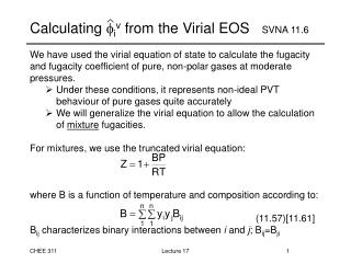
Calculating iv from the Virial EOS • We have used the virial equation of state to calculate the fugacity and fugacity coefficient of pure, non-polar gases at moderate pressures. • Under these conditions, it represents non-ideal PVT behaviour of pure gases quite accurately • The virial equation can be generalized to describe the calculation of mixture properties. • The truncated virial equation is the simplest alternative: • where B is a function of temperature and composition according to: • (11.61) • Bij characterizes binary interactions between i and j; Bij=Bji Lecture 11
Calculating iv from the Virial EOS • Pure component coefficients (B11≡ B1, B22≡ B2,etc) are calculated as previously and cross coefficients are found from: • (11.69b) • where, • and • (11.70-73] • Bo and B1 for the binary pairs are calculated using the standard equations 3.65 and 3.66 at Tr=T/Tcij. Lecture 11
Calculating iv from the Virial EOS • We now have an equation of state that represents non-ideal PVT behaviour of mixtures: • or • We are equipped to calculate mixture fugacity coefficients from equation 11.60 Lecture 11
Calculating iv from the Virial EOS • The result of differentiation is: • (11.64) • with the auxilliary functions defined as: • In the binary case, we have • (11.63a) • (11.63b) Lecture 11
6. Calculating iv from the Virial EOS • Method for calculating mixture fugacity coefficients: • 1. For each component in the mixture, look up: • Tc, Pc, Vc, Zc, • 2. For each component, calculate the virial coefficient, B • 3. For each pair of components, calculate: • Tcij, Pcij, Vcij, Zcij, ij • and • using Tcij, Pcij for Bo,B1 • 4. Calculate ik, ij and the fugacity coefficients from: Lecture 11