Reliability Overview
Reliability Overview. Brad Beaird Last revised 30 June 2014. Agenda- Reliability Overview After completing this module, you will be able to : Understand the role of reliability in design S et system reliability goals A llocate reliability in a design to subsystems


Reliability Overview
E N D
Presentation Transcript
Reliability Overview Brad Beaird Last revised 30 June 2014
Agenda- Reliability Overview • After completing this module, you will be able to: • Understand the role of reliability in design • Set system reliability goals • Allocate reliability in a design to subsystems • Conduct Weibull life analysis • Construct/evaluate test plans
Definition RELIABILITY is . . . • Probability that a component or system will not fail (probability of survival) • Under specified operating conditions • Through a given point in time, R(t)
Quality over Time R(t) at C% confidence Reliability: It’s About PERFORMANCE over Time Reliability The Probability “R” that the item will perform its intended function Confidence The chance “C” that the reliability will be as good as specified Time At what point in time “t” do we need to specify operation? Tools What analyses and tests allow us to make the prediction? How will my design operate over time?
Reliability not modeled, predicted or verified in the development process is left to the customer to determine!!
Key Takeaways: • Reliability testing without testing to failure provides little benefit • Durability measures how long a product will last until it cannot be repaired. Reliability measures intermittent interruptions during this usage period. • We can estimate durability from a reliability test but not the other way around • We should test similar to the customers’ environment • The customers’ experience is based primarily on reliability • Reliability tests are shorter and more efficient than durability tests Reliabilityversus Durability
Reliability Concepts Typical “Quality Over” Time follows a Bathtub Curve Failures Wearout Infant mortality Useful Life Time Reduced through burn-in testing, quality control, error-proofing Initially, failures are due to problems in Workmanship or poor quality control Then, most systems reach a constant rate; failures are caused by environment, chance events Finally, systems wearout, failures are caused by fatigue, corrosion, aging Reduced by design, redundancy Reduced by derating, PM, parts replacement, design technology
Quiz- Reliability Concepts Failures Time • Define reliability • In the infant mortality phase of the bathtub curve, the failure rate is: • Increasing • Decreasing • Constant • In the wear-out phase of the bathtub curve, the MTBF is: • Increasing • Decreasing • Constant
Reliability Planning & Goals • No goal worst case • “As good as current” also pretty lousy • MTBF > 1000 hours a quantified goal for overall system • MTBF > 1000 hours, with 90% confidence even better, speaks to sample size • B10 life (time at which 10% of population will fail) > 1000 hours with 95% confidence for a 90th percentile user Yes! Very specific, measurable, stated in terms of customer usage
Reliability Goals & Growth – MTBF example Given the following field trial data, estimate the MTBF: UnitDaysComment 1 61 failed 2 35 failed 3 59 failed 4 8 failed 5 90 suspended Exercise: Calculate the Mean time between failures (MTBF) The previous series of field tests revealed an MTBF of 50. Is there growth in this reliability parameter?
Reliability Goals & Growth Given the following program test data, calculate and plot the cumulative mean time between failures: Test HoursRepairs/FailuresCumulative MTBF 0-100 12 100/12 = 8.3 hours per failure 101-200 7 200/19 = 10.5 201-300 4 300/23 = 13.0 301-400 3 400/26 = 15.4 401-500 3 500/29 = 17.2 • Called a “Duane” model, can be plotted on a log-log scale to straighten out the line • Alternatively could have plotted the reciprocal failure rate (e.g., failures per 100 hrs) • Will we achieve the goal by the end of the program after 800 hours of testing? Program MTBF goal = 22 Growth parameter
Reliability Allocation-Example System goal could also have been an MTBF figure Car Engine, needs R= 0.90 at 1000 hrs(i.e., B10 > 1000 hrs) System Level Engine Block subsystem R = 0.925 Subsystem Level Fuel & Air subsystem R = 0.973 Component Level Fuel Injector component R=0.995 Connecting Rod component R=0.999 Reliability Allocation is about cascading down a System goal into subsystems & components. Q: Why do numbers get bigger at lower levels of the model?
Reliability Block Diagrams, Series R1= 0.95 R2= 0.97 R3= 0.99 What is the system reliability? Reliability of System= 0.95 x 0.97 x 0.99 = 0.91 We use Reliability Block Diagrams to model our system from the bottom up using estimates on components and subsystems
Reliability Block Diagrams, parallel R1= 0.75 R3= 0.99 R2= 0.75 We can design using redundant, relatively low reliability components in parallel to achieve overall system reliability goals What is the system reliability? Hint: Figure out the parallel subsystem reliability, then multiply in series with component 3.
Reliability Block Diagrams, Parallel (redundancy) R1= 0.75 R3= 0.99 R2= 0.75 RS= [1-(1-R1)(1-R2)] x R3 = [1-(0.25)2] x 0.99 = 0.9375 x 0.99 =0.928 The trick for this subsystem reliability is: Probability (subsystem survives) = Probability (1 or more survives) = 1 – probability (R1 and R2 fail) = 1 – 0.252
Reliability Block Diagrams- Exercise R= 0.90 R= 0.85 R= 0.90 R= 0.95 R= 0.90 R= 0.92 Calculate the reliability of this system
Reliability Allocation Exercise R= 0.90 R= ? R= 0.90 R= 0.95 R= 0.90 R= ? Q: If the overall system reliability goal is 0.98, what should the reliability be for the two redundant components in the far right subsystem? Assume both components have the same reliability.
History on Weibull • WaloddiWeibull- Swedish Engineer • Famous for pioneering work on reliabilityand life analysis • The Weibull distribution is named after him, and is a popular tool for modeling lifetimes
Types of Functions Reliability or Survival Function Cumulative Distribution Function Probability Density Function Hazard Function
More on The Weibull Distribution • Well suited for modeling lifetime data • Components • Systems • Parameters • Slope of the line (shape, β) • Characteristic life (measures dispersion of data, ), B63.2 life • Optional, guaranteed life (time before anything will fail, ) • Mimics many distribution shapes (skewed left, skewed right, symmetric) • Characterizes the failure distribution so we can make predictions • Tells us where we are in the bathtub curve so we can fix problems Weibull Reliability equation β<1 means infant mortality, β=1 means useful life, β>1 means wear-out
Weibull Reliability Practice Calcs Weibull Reliability equation
Example Weibull analysis B10 – Point at which 10% of failures predicted 3 hours 1 2 3 4 5 6 789 10 20 30 40 50
Information We Can Get From Completed Plot We can compare two products or processes Example- compare components from 2 suppliers Q: Which one is “better” (hint- it’s an open-ended question) 1 2 3 4 5 6 789 10 20 30 40 50
Information We Can Get From Completed Plot DV1 We can show objective evidence of reliability GROWTH DV2 On the Weibull plot, “growth” means pushing the plotted line to the right and flattening it 1 2 3 4 5 6 789 10 20 30 40 50
Weibull Analysis Exercise • Statement on GE light bulb package: Lifetime 1000 hrs(what does this mean?) • Data (time to fail) • 450 hrs • 2100 hrs • 1200 hrs • 805 hrs • What is the slope? • What is the characteristic life? • What is the B10 life? B50 life? • What part of the bathtub curve are we in? Let’s do Weibull Analysis by hand to understand the technique Gather data & sort in ascending order Get median rank values from table Plot ordered pairs (time, median rank) Fit a straight line Estimate distribution parameters
Looks like the GE figure of 1000 hours is a median (B50) life
Previous MTBF example Given the following field trial data, estimate the MTBF: UnitDaysComment 1 61 failed 2 35 failed 3 59 failed 4 8 failed 5 90 suspended • Weibull gives much more info than MTBF alone • We can characterize the entire life distribution • When we have suspended data (like unit #5 above), software is usually used to do the Weibull analysis
Accelerated Life Testing Example • We can mimic the life of our product in the field via testing • Problem is we only have a short time to test for a long life • Solution accelerate the testing via higher stresses: • Stress in this example is temperature • We ran tests to fail at 4 higher temps and did Weibull analysis • We then predicted the life at a normal temp of 80 degrees
System Maintenance Applications • Used to determine optimal parts replacement strategies • The approach • Collect time to fail data, construct a Weibull plot, and verify you are in the wear-out phase of the bathtub curve. • The optimal time to replace a part is based on Weibull parameters and ratio of cost of unplanned maintenance to planned maintenance. • Overall goal is to reduce total cost of downtime and improve system availability. Availability = MTBF/ (MTBF + MTTR). • To improve system availability, you either increase the mean time between failures or decrease the mean time to repair or both.
System Availability, Exercise • If MTBF = 100 hours and MTTR = 24 hours, A = ? • If MTBF = 200 hours and MTTR = 24 hours, A = ? • If MTTR = 24 hours and Availability goal = 0.97 (97%), MTBF = ?
Zero Failure Acceptance Testing Acceptance testing (versus testing to failure) is sometimes necessary, though we do not learn as much. • Calculate Exercise: The requirement for a component states that the supplier must demonstrate at least 95% reliability with 90% confidence (R95 C90). How many units should the supplier test with no failures in order to pass?
Exercise- Demonstration Testing Customer acceptance criteria requires us to demonstrate a B10 life > 500 hours, with 95% confidence. Past testing shows the Weibull slope is 1.6. There is 1000 hours available in the test lab. How many units must be tested, with zero failures allowed? β=1.6 Confidence = 95% (0.95) R= 0.90 (B10 90% reliability) Target time= 500 hrs, Actual time=1000 hrs, k is multiple of required time n=
Agenda- Reliability Overview • Our learning objectives were: • Understand the role of reliability in design • Set system reliability goals • Allocate reliability in a design to subsystems • Conduct Weibull life analysis • Construct/evaluate test plans Do you understand? Questions?