Download
1 / 19
190 likes | 317 Vues
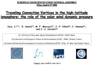
EUROPEAN GEOSCIENCES UNION GENERAL ASSEMBLY Wien, April 2-7 th 2006. Traveling Convection Vortices in the high-latitude ionosphere: the role of the solar wind dynamic pressure. Coco, I. (1*) , E. Amata (1) , M. F. Marcucci (1) , J.-P. Villain (2) , C. Hanuise (2) , and J.-C. Cerisier (3).

E N D
EUROPEAN GEOSCIENCES UNION GENERAL ASSEMBLY Wien, April 2-7th 2006 Traveling Convection Vortices in the high-latitude ionosphere: the role of the solar wind dynamic pressure Coco, I.(1*), E. Amata(1), M. F. Marcucci(1), J.-P. Villain(2), C. Hanuise(2), and J.-C. Cerisier(3) • Istituto di Fisica dello Spazio Interplanetario (IFSI) – INAF, Roma. • (2) Laboratoire de Physique et Chimie de l’Environnement (LPCE) – CNRS, Orléans, France. • (3) Centre d’Etude des Environnements Terrestre et Planétaires (CETP) – IPSL, St. Maur des Fossés, France. * Contact: igino.coco@ifsi-roma.inaf.it
Abstract: Traveling Convection Vortices (TCVs) are one of the most interesting and controversial phenomena in the framework of the studies on the solar wind, magnetosphere and ionosphere coupling. Their origin, and their actual contribution to the energy transfer from the solar wind and the upper atmosphere are still subject of debate. We present here signatures of TCVs in the Northern polar cap observed after an interplanetary shock hit the Earth's magnetosphere on 6 January 1998 at 14:15 UT. Three main features emerge from observations in space: 1) the shock wave front is tilted towards dawn; 2) IMF data show appreciable differences between L1 (WIND and ACE data) and just upstream of Earth's bow shock (IMP-8 data); 3) After the main shock, three minor pressure jumps are observed. The TCV dynamics is studied with both ground magnetometers and SuperDARN data. Two main vortices systems show up: a couple of vortices in the morning side, traveling towards noon, and a single vortex in the afternoon. Hints of shorter-life traveling vortices are seen in the morning, after the passage of the main TCV system. The interplanetary shock should definitively be the cause of the ground signatures, but the scenario is very complex and not univocally associable to one existing model. A brief discussion is included.
Zesta et al., JGR, 107, 1317, 2002 Transient Convection Phenomena (1) In the magnetosphere... In the ionosphere... Sibeck, JGR, 95, 3755, 1990 magnetopause perturbation induced magnetospheric vortices Field Aligned Currents Travelling Convection Vortices (TCV) (example for eastward propagation) Possible causes: solar wind dynamic pressure pulses, Kelvin – Helmholtz instability, impulsive plasma penetration, patchy or sporadic reconnection...
Transient Convection Phenomena (2) MHD Wave MP Bow shock DAWN DUSK Shock front To Sun Alfvén waves SC - Morning SC - Afternoon Current System of the PI of a SC. The Araki Model When an interplanetary shock hits the magnetopause a fast compressional MHD wave is launched. Due to plasma density inhomogeneities always present in the magnetosphere, the MHD wave couples with transverse Alfvén waves which propagates along the geomagnetic field lines down to the polar ionosphere, carrying with them Field Aligned Currents (FAC). Following Araki, Geophys. Monogr., 81, 183, 1994, an incoming FAC is driven in the afternoon, and an outcoming one in morning. The ground signatures of this couple of FACs are two convection vortices, one counterclockwise in the morning and one clockwise in the afternoon... ...When the shock wave has passed away, the magnetosphere reaches a new equilibrium configuration, another couple of FACs is induced with opposite polarity with respect to the previous one, and the circulation of the vortices is reversed. The magnetometer signature of such phenomena is called “Sudden Commencement” (SC), and the two vortices systems lead to a double-impulse feature, where a Preliminary Impulse (PI) preceeds the Main Impulse (MI).
SuperDARN (Super Dual Auroral Radar Network) 1 • SuperDARN is a network of radars which work sinchronously and continuously btw 8 and 20 MHz (Greenwald et al., Space Sci. Rev., 71, 761, 1993). • Every radar is composed by 16 antennas spanning a 52° field of view along 16 selected directions (“beams”), with a time resolution of 2 min. • SuperDARN radars provide a direct measure of the plasma convection velocity in the ionosphere, through a time decorrelation of the Doppler signals detected along each beam. • At present, 10 radars are operating in the Northern hemisphere (A) and 7 in the Southern hemisphere (B). • IFSI-INAF (Italy) and LPCE – CNRS (France) manage the Kerguelen radar (red shaded area in Fig. B). The construction of two new radars at Dome C, Antarctica, is scheduled for the 2007/2008 Franco-Italian antarctic campaign.
SuperDARN (Super Dual Auroral Radar Network) 2 Examples of observations • Example of a complete scan of the Stokkseyri radar, Iceland (January 6, 1998, 14:16 – 14:18). A direction (beam) given, 75 azimuthal ports are sounded, up to 3000 km from the radar site. Following the color scale in the figure, positive velocities (blue to violet) mean fluxes directed towards the radar, negative velocities (red to yellow) mean fluxes directed away from the radar, along the line of sight. The red dotted line marks the direction of beam 8. • Another way to display SuperDARN data: RTI plots. A beam is fixed, and the time series of the velocity, as a function of the distance from the radar, is shown. Here we can see data from beam 8 for January 6, 1998, 14 – 15 UT: between the two red dotted lines, data for the two-minutes scan shown above (14:16 – 14:18) are displayed.
IMF z y SuperDARN (Super Dual Auroral Radar Network) 3 Global Convection Maps In the picture, the line-of-sight velocities of all the available radars in the Northern hemisphere are fitted to the transpolar equipotential curves, through a spherical harmonic expansion of the polar potential following the relations: E = - , V = (E X B)/B2 (Ruohoniemi & Baker, JGR, 103, 20797, 1998). Where data coverage is poor, a model is superimposed based on statistical values of the potential depending on IMF conditions (Ruohoniemi & Greenwald, JGR, 101, 21743, 1996). The inset on top right shows the IMF vector in the GSM YZ plane (as measured by IMP 8 spacecraft), color scale on top left represents the intensity of the velocity vectors. Coordinates are Altitude Adjusted Corrected GeoMagnetic (AACGM, Baker & Wing, JGR, 94, 9139, 1989).
IMF IMF z z y y SuperDARN convection maps, 06/01/1998 – 14:14 14:18 TU Between 14:16 and 14:18 UT, SuperDARN radars see a double-vortex system in the morning (evidenced in blue). The centres of the vortice lie between 75° and 77° Mag. Lat. The eastern vortex is counterclockwise, which means that it has been formed by an incoming FAC, the western is clockwise, which implies an upcoming FAC. A possible hint of a clockwise vortex emerges in the afternoon too.
IMF IMF z z y y SuperDARN convection maps, 06/01/1998 – 14:18 14:22 TU The vortices system in the morning persists until 14:22 UT. In the afternoon, a clockwise vortex is clearly seen.
IMF IMF z z y y SuperDARN convection maps, 06/01/1998 – 14:22 14:26 TU Between 14:22 and 14:24 the afternoon vortex is still present, while in the morning we can see a weavy perturbation of the equipotential curves, which leads to think to vortical structures moving tailward. The bending of the curves and the propagation effect are still clearer between 14:24 and 14:26 (picture on the right).
Morning Sector (Magnetic Local Time 06 - 12) I MACCS* magnetometers and SuperDARN convection maps comparison. At 14:22 UT the vortex centre is found at about 10 MLT, roughly keeping the same mag. Lat. Looking at the magnetograms below, we can estimate the vortex centre speed to be about 13 14 km/s. The vortex is travelling towards noon. Starting from 14:16 UT, MACCS magnetometers clearly show a double TCV signature. SuperDARN radars are able to follow the evolution of one vortex at least. In the convection maps, the vortex is seen at first btw 14:16 and 14:18 UT, with centre around 75° mag. Lat. and 8 MLT (red circle in fig. below). RBY X RBY X 100 nT 100 nT RBY Y RBY Y CDR CDR V 13 14 km/s CHB CHB CHB X CHB X RBY RBY CHB Y CHB Y CDR X CDR X CDR Y CDR Y *We aknowledge M. Engebretson e W. J. Hughes at Boston University for the use of MACCS data.
Morning Sector (Magnetic Local Time 06 - 12) II IMF IMF IMF IMF z z z z y y y y CDR CDR CHB CHB CDR CDR CHB CHB V 5 6 km/s Starting from 14:22 UT, a series of three magnetic pulses is seen around 75° mag. lat. and 9 MLT. The period is 4-5 minutes. SuperDARN convection maps show vortical structures moving tailward. This tailward motion is confirmed also by the magnetometers (see figure above), and the estimated speed is about 5-6 km/s.
Afternoon Sector (Magnetic Local Time 12 - 18) DMI* and MAGIC** magnetometers and SuperDARN convection maps comparison Similarly, magnetometers in Greenland observe a clockwise vortex starting at 14:16 UT. Following the SuperDARN maps (which begin to observe the vortex somewhat later, at 14:18 UT), the vortex centre can be placed at ~ 75° mag. lat and 13-14 MLT. From magnetometers data it is not possible to clearly detect any hint of vortex motion. Looking at SuperDARN maps, it seems the vortex is moving tailward, but we cannot be sure of that: IMF Bz has become negative, the whole convection cell is expanding and this should result in an apparent vortex expansion and motion. GDH H GDH H 50 nT 50 nT GDH E GDH E GDH GDH MCG MCG MCG H DNB MCG H DNB MCG E MCG E DNB H DNB H DNB E DNB E 14:22 – 14:24 14:18 – 14:20 * Courtesy of J. Watermann at Danish Meteorological Institute ** Courtesy of R. Clauer at Michigan University
To Sun 2 1 Further considerations... A magnetosphere picture made by the OVT program (http://ovt.irfu.se), using the Tsyganenko 96 Model of the Earth’s magnetic field with realistic values of IMF, solar wind pressure and Dst index, for January 6, 1998, 14:20-14:22 UT. Two field lines have been projected from 2 magnetometer stations at ground to the magnetopause region (bullet-shaped shaded area in the figure). Lines 1 and 2 have footprints at CHB and CDR stations, in the morning: they never cross the magnetopause and their distance, in the region closest to the magnetopause is about 2 RE. The delay of the ground signature btw the two stations is in good agreement with a solar wind propagation velocity of about 350 km/s. The Spectral Width (SW) measured by the SuperDARN radars is the width of the velocity distribution for each cell. It has been demonstrated (Baker et al., JGR, 100, 7671, 1995), that regions corresponding to the ionospheric footprints of the Cusp and LLBL are characterized by high values of the SW. In the figure a red line has been plotted in the morning side, following a sharp transition btw regions of lower and higher SW. This line can be considered as a good proxy of the so-called “Open-Closed field lines Boundary” (OCB). For that period, in the morning side, the OCB can be placed around 75° mag. lat.
WIND data*. 6 january 1998. 13:29 UT From top to bottom (GSM): |B|, Bx, By, Bz, V, Dynamic Pressure. Mag. field data res.: 3 sec. Plasma data res.: 1 min. 13:29 UT: a sharp discontinuity is observed in the IMF data. The plasma dynamic pressure has a jump of about 6 nPa and the velocity has an increase of about 80 km/s. Density oscillations with period of ~ 6 8 min. *We aknowledge R. P. Lepping and K. W. Ogilvie for the use of IMF and plasma data of WIND.spacecraft.
IMP-8 GOES-9 GOES-8 Wind y Ace GEOTAIL SI front, 14:13 UT φ n x WIND (RE):X=227, Y= 20, Z =-2 ACE (RE): X=220, Y= 32, Z =-5 IMP 8 (RE): X=29, Y=-1, Z=14.6 GEOTAIL (RE):X= 7, Y=6, Z=0.5 GOES-8: geostat. ~ 9 MLT GOES-9: geostat. ~ 4 MLT Normal calculation (coplanarity): φ = -28° ± 4° θ = -7° ± 3° Vsh = 379 ± 7 km/s Using both plasma and IMF high resolution (3 secs) data from WIND spacecraft, and following the Coplanarity Theorem (the shock normal, n, the magnetic field and the velocity on both sides of the shock, all lie in the same plane), we calculated the shock normal orientation, and found the shock is tilted toward dawn by roughly 30°, as shown in the figure above. The shock velocity along the normal direction is about 380 km/s.
GEOTAIL* IMP 8* GOES – 8* GOES - 9 Arrival times of the shock at WIND, ACE and IMP 8. The “Calculated” column shows the delays between couples of satellites, as results from the coplanarity analysis: Blue: SI at GEOTAIL 14:16:10 Red: magnetopause at GEOTAIL ~14:19 The observed and calculated delays agree in the limits of the errors: the shock wave hits first the dawn-side magnetopause possibly around 14:15 UT. At GOES-8 (~ 9 MLT) a step-like increase of Bz is reported at 14:15:55. GEOTAIL lies close to the afternoon magnetopause, in the equatorial plane, and noticed a field compression at 14:16:10. After a while, the spacecraft crosses the magnetopause (~ 14:19). NOTE: the interplanetary magnetic field as observed by IMP 8 (middle panel) shows important differences with respect to the WIND observations; above all, at the IMP 8 position, IMF Bz > 0 when the shock arrives. 14:13:20 Black: SI at IMP8 14:15:55 Green: SI at GOES-8 *We aknowledge S. Kokubun, A. Szabo, R. P Lepping and H. Singer for the use of magnetic field data of GEOTAIL, IMP8 and GOES spacecraft.
Resuming the observations... • An interplanetary shock is observed by WIND at 13:29 UT; it reaches the Earth’s magnetopause around 14:15 UT, in the morning side. Such pressure pulse is followed by density oscillations of minor intensity. • Starting from 14:16 UT, almost contemporarily in the whole day side, magnetometers observe vortices systems, whose centres are located around 75° magnetic latitude, which corresponds to the OCB latitude for that event. • Looking at magnetometers data, two different vortices systems seem to show up: a single clockwise vortex in the afternoon, for which no clear motion can be detected, and a double vortex system (counterclockwise/clockwise) in the morning, moving eastward (toward noon), with speed of about 13 14 km/s. • Both systems are observed by SuperDARN radars, which confirm a counterclockwise plasma motion (which means upcoming FACs) for the first morning vortex, and a clockwise plasma motion (which means downcoming FACs)for the second morning vortex and the afternoon vortex. The morning vortex centre is clearly moving toward noon, which is very rare: one should expect an antisunward motion instead. • On the other hand, the behaviour of the afternoon vortex is quite different: this vortex is not generated by the same FACs system which operates in the morning, because it appears at the same time, with the same circulation sense of the second morning vortex (very far from there) and seems not moving at all. • Starting from 14:22 UT, at least three transient signatures are observed by MACCS magnetometers, around 75° mag. lat., each one lasting for about 5 minutes, and moving tailward with a speed of about 5-6 km/s. SuperDARN convection maps show vortical structures in that region.
Conclusions • We can conclude that the solar wind pressure pulse is the cause of all the observed ground signatures. • We think the tilt of the interplanetary shock may play an important role in the morning vortices system behaviour: the magnetopause compression is asymmetric and the footprints of the FACs induced in the morning are first dragged towards noon and then towards the tail, following the solar wind discontinuity propagation. For that reason, the morning TCVs are seen moving toward noon. • Models of the kind proposed by Sibeck (Sibeck, JGR, 108, 1095, 2003) seem to explain the couple of vortices in the morning. Their centres map close to the magnetopause, but probably still inside the magnetosphere: the pressure enhancement induces a bulge in the magnetopause surface, and FACs are induced where the pressure gradients change, for example near the inner edge of the LLBL; the signs of the FACs that we deduce from the vortices circulation are those expected from the model. • At the same time, a more global effect seems to be superimposed, of which the vortex we see in the afternoon is an evidence. The magnetometers signature over Greenland is that expected from Araki model in the afternoon: a negative Preliminary Impulse followed by a positive Main Impulse. At some station, expecially in the East coast, this signature is quite broad and the PI lasts for more that 5 minutes, while the predicted signature for the PI should be narrower. Nevertheless, for tilted shock fronts, it has been demonstrated that the ionospheric response could be delayed and broadened (Takeuchi et al., JGR, 107, 1423, 2002). SuperDARN data confirm this picture, and show a clockwise vortex lasting for about 6 minutes. • The minor pressure variations that follow the main interplanetary shock, give rise to a series of traveling vortices in the morning, whose direction is tailward, i.e. opposite with respect to the previous TCV system. We did not investigate this aspect in major detail, but it seems reasonable to think that such solar wind “buffetings” are no more related to the shock structure: IMF has considerably changed, and the new pressure variations should be part of a new solar wind structure, with an orientation that could be rather different with respect to that of the shock.