Complete Random Design
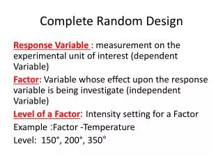
Complete Random Design. Response Variable : measurement on the experimental unit of interest (dependent Variable) Factor : Variable whose effect upon the response variable is being investigate (independent Variable) Intensity setting for a Factor : Level of a Factor

Complete Random Design
E N D
Presentation Transcript
Complete Random Design Response Variable : measurement on the experimental unit of interest (dependent Variable) Factor: Variable whose effect upon the response variable is being investigate (independent Variable) Intensity setting for a Factor :Level of a Factor Factor -Temperature:Example °Level: 150°, 200°, 350
Complete Random Design Treatment: a combination of factor levels applied to an experimental unit Example: Factors-Temperature , Time, Humidity Treatment-temp at 150, time at 10 min, Experimental Design : the selection of treatments to be studied and the plan for randomly assign treatment to experimental units
Complete Random Design CRD: the treatments are randomly allocated to the N homogeneous experimental units in such a way that n1 units receives trt1, n2 receives trt2,…., narecivestrta Note: In the CRD, there are no restrictions on the random assignment of treatments except that each treatment is to be assigned to a specified # of units.
From book))Example Response: Etch rate Factors Power settings Treatments power at 16, 180… Design Randomize Design Level of factors 160, 180, 200, 220
Complete Random Design Fixed Effect: inference is to be on the a treatment only Random Effect: The treatments are randomly selected from a large population of treatments with inference to be on all treatments in the population
Analysis of Variance :One way classification (ANOVA) Purpose: make an inference on , µ1, µ2,…, µa Where a= # of populations H0:µ1= µ2=…= µa Assumptions: All population are normally distributed Equal but unknown variances Random sample taken from each population Independent Sample
ANOVA Data:
ANOVA ANOVAs Philosophy? Why is called Analysis of variance when H0:µ1= µ2=…= µa Plot the population when a=3 If Ho is true then
ANOVA ANOVAs Philosophy? Why is called Analysis of variance when H0:µ1= µ2=…= µa Plot the population when a=3 If H1 is true then
ANOVA When considering the total variability in There are two sources of variability • Variability within sample • Variability between samples (caused by different means) ANOVA Philosophy –Compare variance between and within samples to make inferences on population means.
The CRD Model • Mean Model: • Model: • Assumptions :
Analysis of Fixed Effect Model Model Note: the above model has the same assumptions made for one way ANOVA (Normal population, independent, random sample)
Connection between Mean Model and One-way ANOVA Model • Mean Model has a Parameters and ANOVA has a+1 parameters , therefore we may impose one constraint on the parameters of the model
Testing the hypothesis H0:µ1= µ2=…= µa H1: at least one pair are not equal
Contrast • When the Ho hypothesis was rejected , all what we know that there is difference among treatments but which one actually cause this different. Therefore we make multiple comparison methods and we use the idea of contrast
Contrast • For Fixed Effect CRD
Contrast • For Fixed Effect CRD
Contrast • Find E(MSc) ?
Example Continue • Test the difference between µ1 and µ2 • Ho: µ1 = µ2 • H1: µ1≠ µ2 • In Other way Ho: µ1- µ2=0
Example Continue • Ho: µ1=2 µ2 • H1: µ1≠2 µ2
Example • Test the difference between µ1 and µ2 • Ho: µ1 = µ2 • H1: µ1≠ µ2 We conclude fail to reject The Ho hypothesis There is no differences Between the two power 160 and 180 on the etch rate
Example • Test the difference between µ1 and µ2 • Ho: µ1 = µ4 • H1: µ1≠ µ4 We conclude not to reject The Ho hypothesis There is differences Between the two power 160 and 220 on the etch rate
Orthogonal Contrast • Consider the relationship between
Orthogonal Contrast • Define • Note : In the case where are a treatments (sample mean), there are at most (a-1) mutually orthogonal contrast
Orthogonal Contrast • Fact: If C1, C2,…,Ca-1 is a set of a-1 orthogonal Contrast then The variation in data attributed to treatments can be partitioned into parts which can be attributed to various orthogonal contrast